Congratulations, my friends, we have finally come to the end of the series! Although… well, not quite (see below), but we have definitely reached the end of what I had planned originally. Last time, we discussed diffusion-based models, mentioning, if not fully going through, all their mathematical glory. This time, we are going to put diffusion-based models together with multimodal latent spaces and variational autoencoders with discrete latent codes, getting to Stable Diffusion and DALL-E 2, and then will discuss Midjourney and associated controversies. Not much new math today: we have all the Lego blocks, and it only remains to fit them all together.
Diffusion models + VQ-GAN = Stable Diffusion
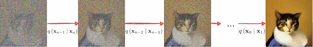
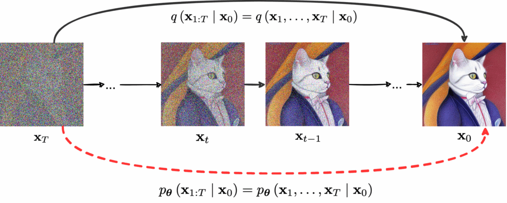
We already know how diffusion-based models work: starting from random noise, they gradually refine the image. The state of the art in 2021 in this direction was DDIMs, models that learn to do sampling faster, in larger steps, but have generally the same final quality.
Then Stable Diffusion happened. Developed by LMU Munich researchers Robin Rombach et al., it was released in August 2022 and published in CVPR 2022 (see also arXiv). Their idea was simple:
- diffusion models are very good at generation but relatively slow and hard to scale up to huge dimensions of real images;
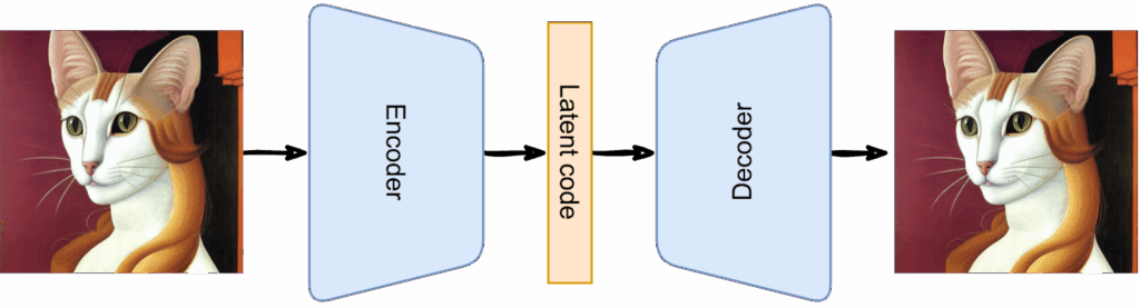
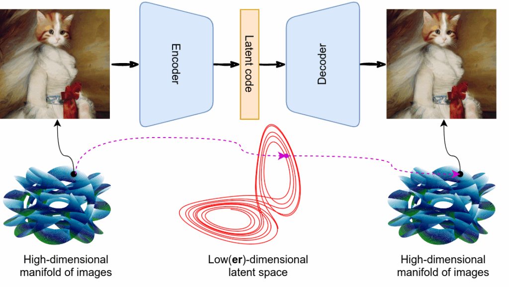
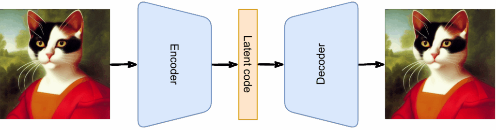
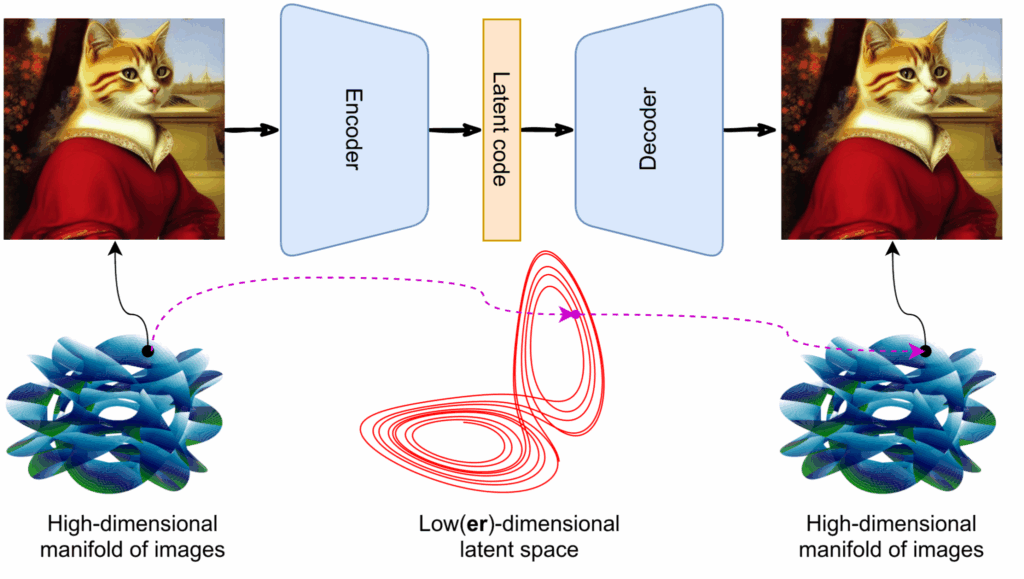
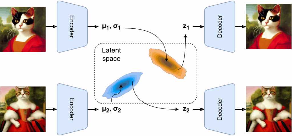
- VAEs are very good at compressing images to a latent space (perhaps continuous, perhaps discrete);
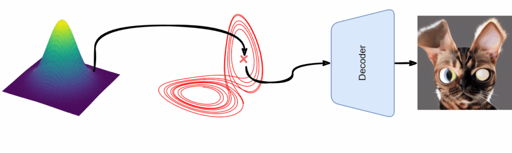
- so let’s use a diffusion model to generate the latent code and then decode it with a VAE!
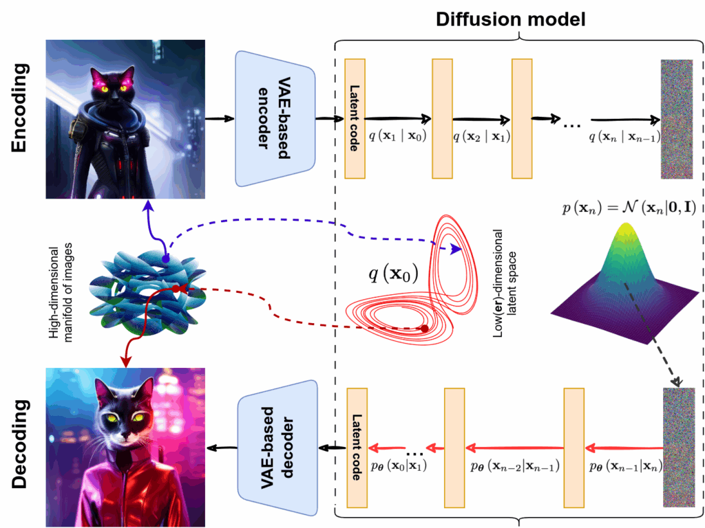
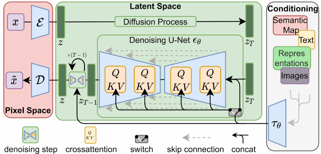
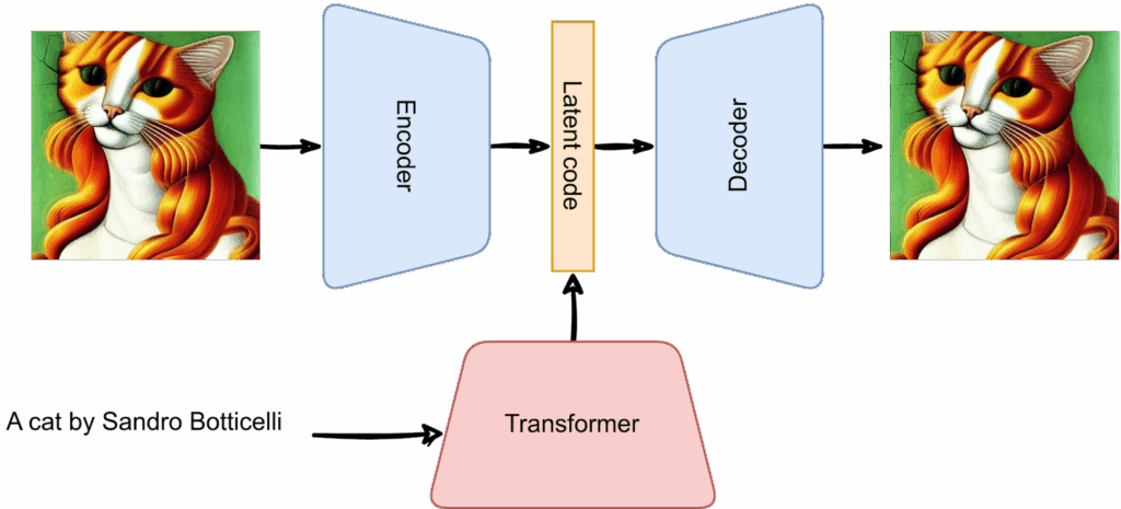
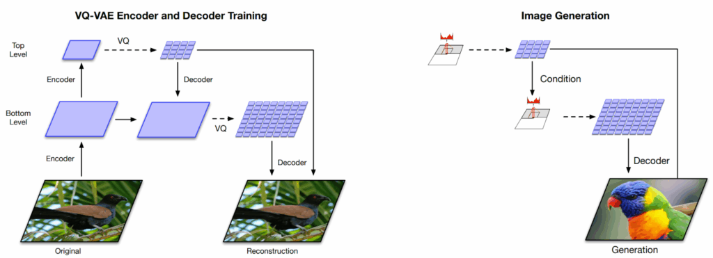
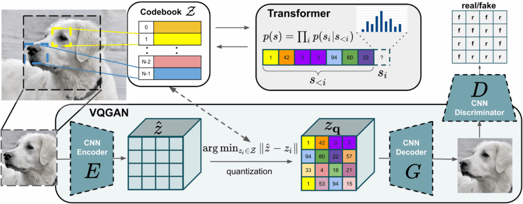
This is basically it: you can train an excellent diffusion model in the low-dimensional latent space, and we have seen that VAE-based models are very good at compressing and decompressing images to/from this latent space. The autoencoder here is the VQ-GAN model that we have discussed earlier.
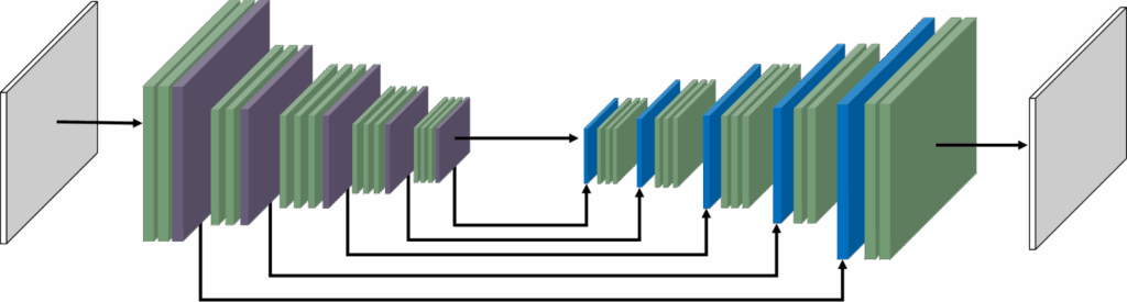
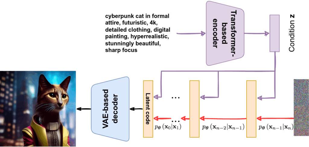
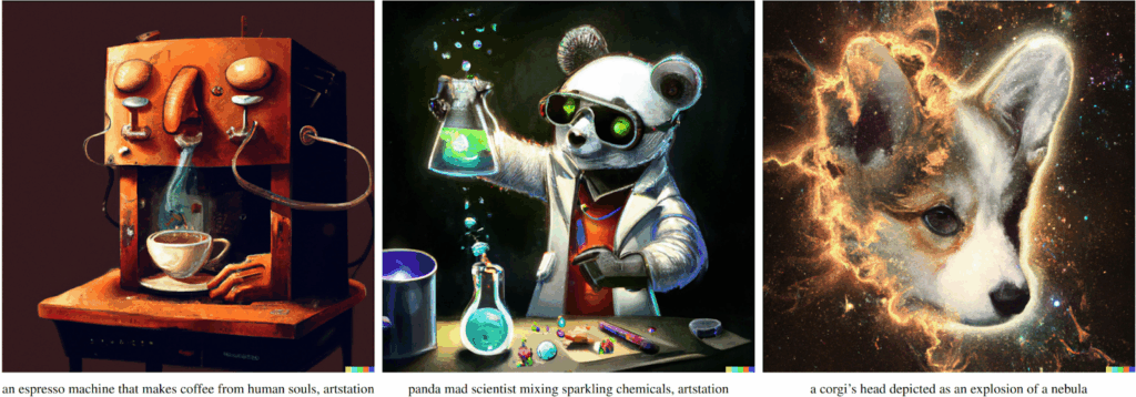
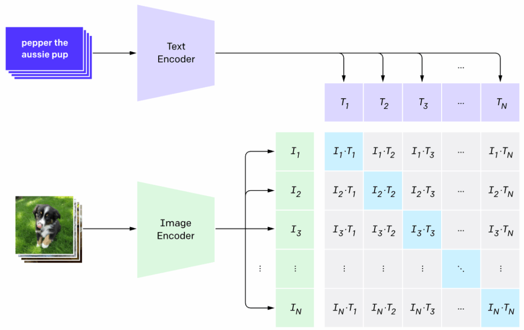
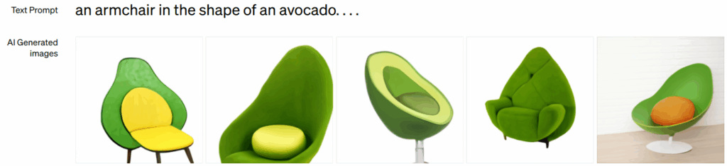
Another novelty of the Stable Diffusion model was a conditioning mechanism. The authors used a U-Net as the backbone for the diffusion part, but they augmented it with Transformer-like cross-attention to allow for arbitrary conditions to be imposed in the latent space. As a result, the condition is introduced on every layer of the diffusion decoder and on every step of the denoising. Naturally, the main application of this is to use a text prompt encoded by a Transformer as the condition:
Stable Diffusion had been released by LMU Munich researchers but soon found itself as the poster child of the Stability AI startup, which recently led to a conflict of interests. The controversy with Stability AI is currently unfolding, and until it is fully resolved I will refrain from commenting; here is a link but let’s not go there now.
Whatever the history of its creation, Stable Diffusion has become one of the most important models for image generation because it is both good and free to use: it has been released in open source, incorporated into HuggingFace repositories, and several free GUIs have been developed to make it easier to use.
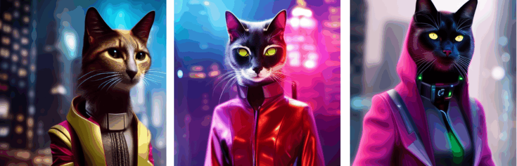
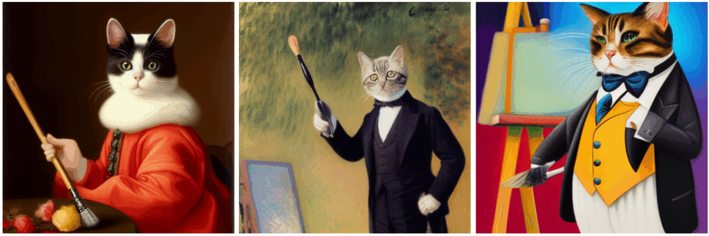
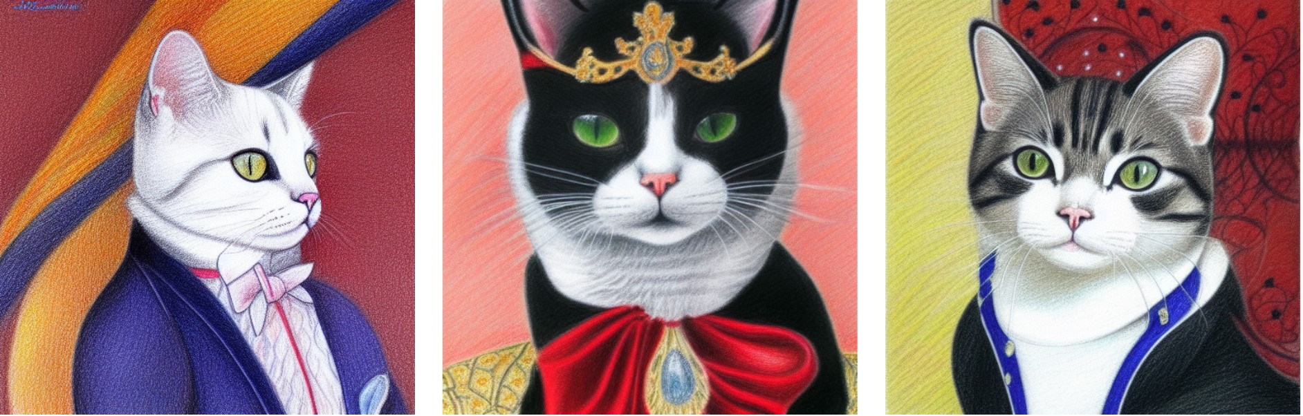
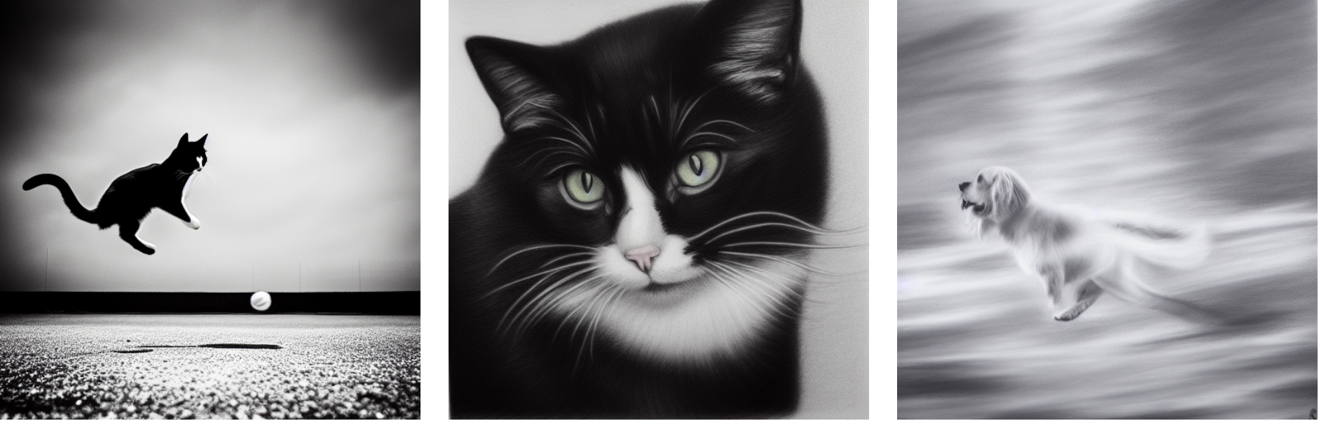
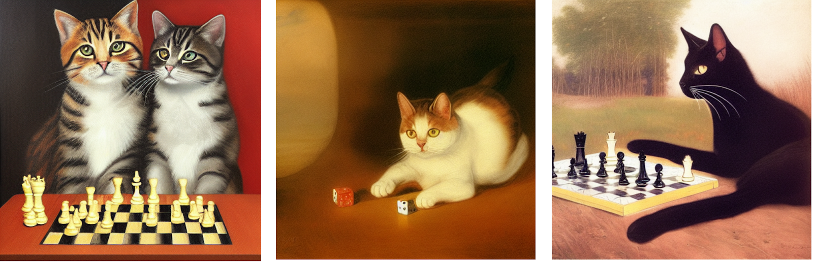
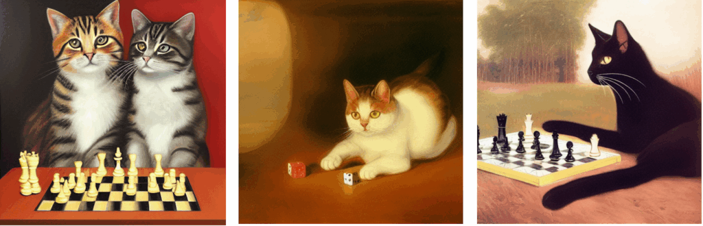
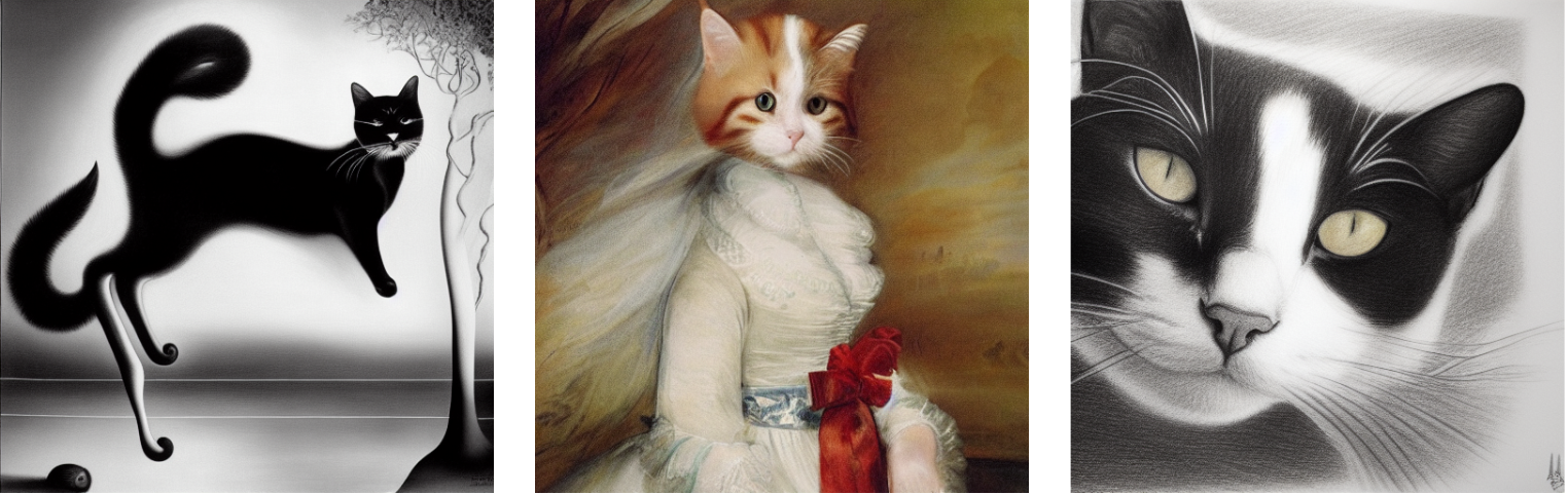
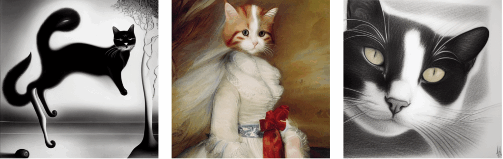
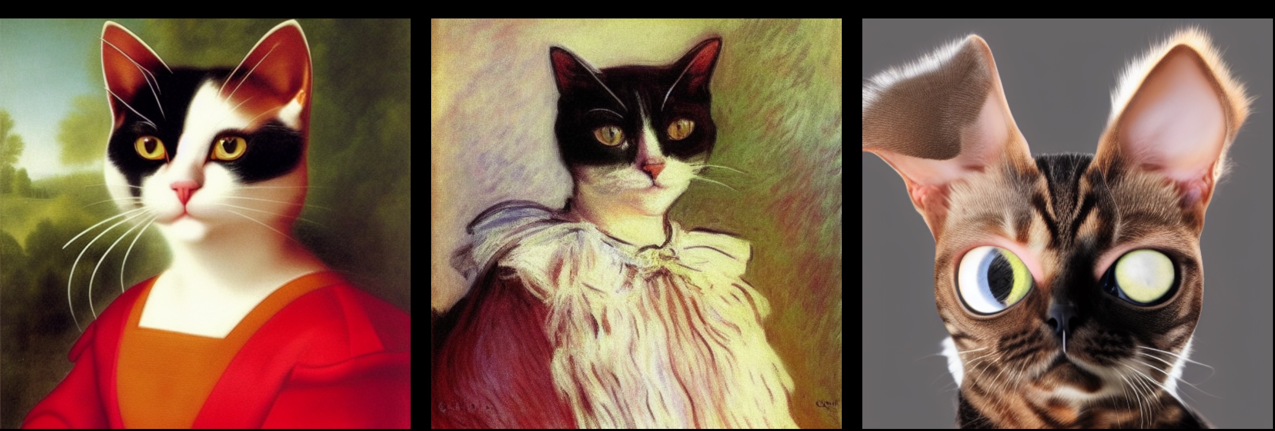
I will not give specific examples of Stable Diffusion outputs because this entire series of posts has been one such example: all cat images I have used to illustrate these posts have been created with Stable Diffusion. In particular, the prompt shown above is entirely real (augmented with a negative prompt, but making prompts for Stable Diffusion is a separate art in itself).
Diffusion models + CLIP = DALL-E 2
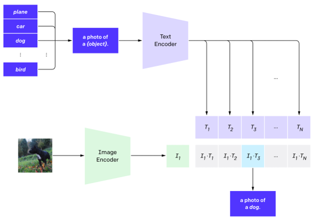
Stable Diffusion uses a diffusion model in the latent space of a VQ-GAN image-to-latent autoencoder, with text serving as a condition for the diffusion denoising model. But we already know that there are options for a joint latent space of text and images, such as CLIP (see Part IV of this series). So maybe we can decode latents obtained directly from text?
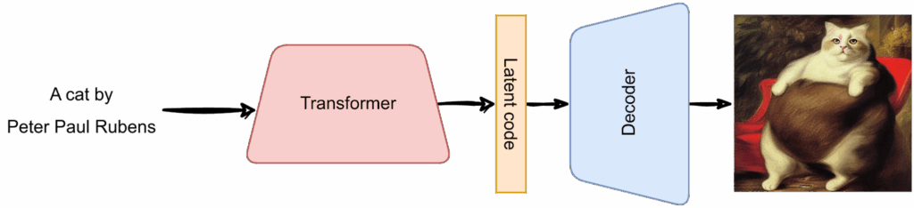
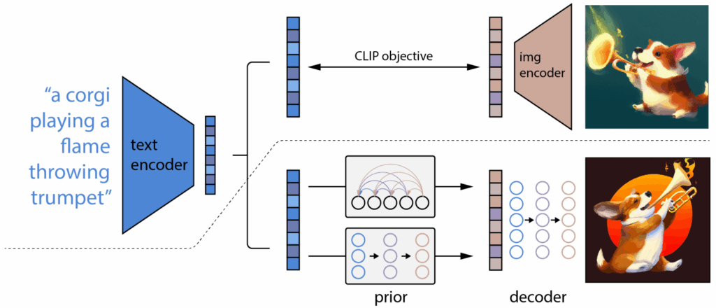
DALL-E 2, also known as unCLIP, does exactly that (Ramesh et al., 2022). On the surface, it is an even simpler idea than Stable Diffusion: let’s just use the CLIP latent space! But in reality, they still do need a diffusion model inside: it turns out that text and image embeddings are not quite the same (this makes sense even in a multimodal latent space!), and you need a separate generative model to turn a text embedding into possible matching image embeddings.
So the diffusion-based model still operates on the latent codes, but now the text is not a condition, it’s also embedded in the same joint latent space. Otherwise it’s the exact same multimodal CLIP embeddings that we discussed in an earlier post. The generation process now involves a diffusion model, which the authors of DALL-E 2 call a diffusion prior, to convert the text embedding into an image embedding:

(This time, the prompt is a fake, it’s a Stable Diffusion image again.)
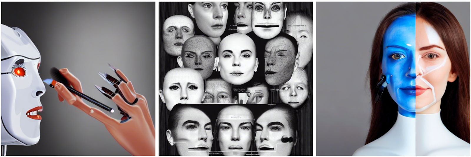
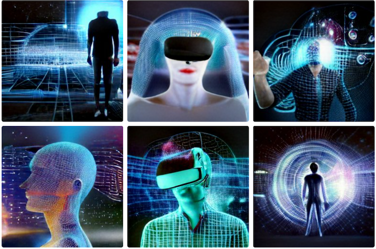
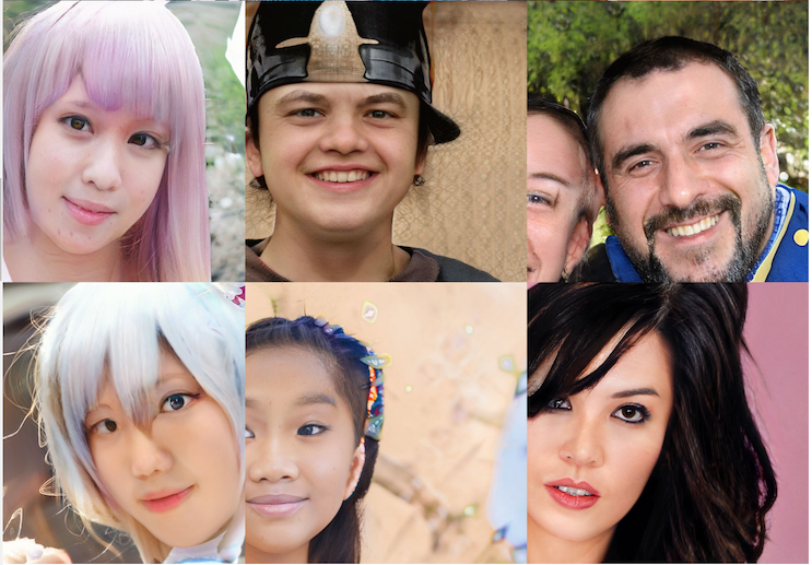
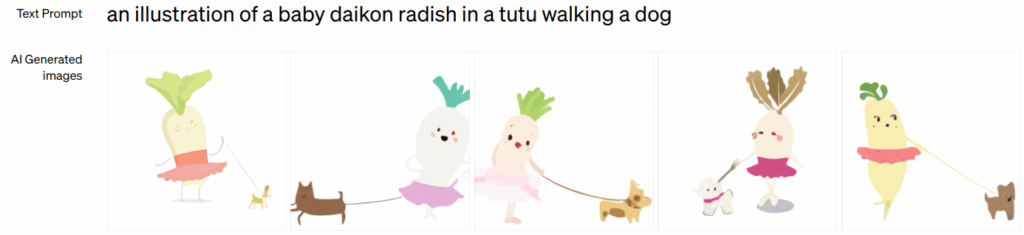
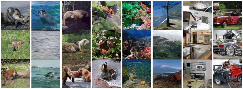
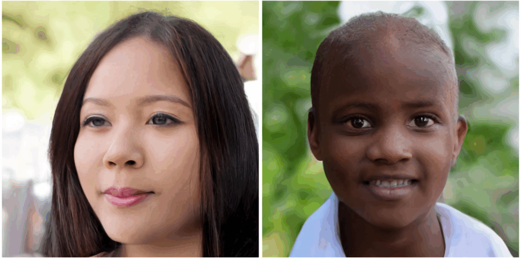
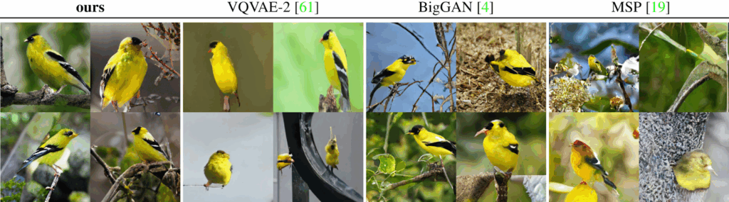
DALL-E 2 reports excellent generation results; here are some samples from the paper:
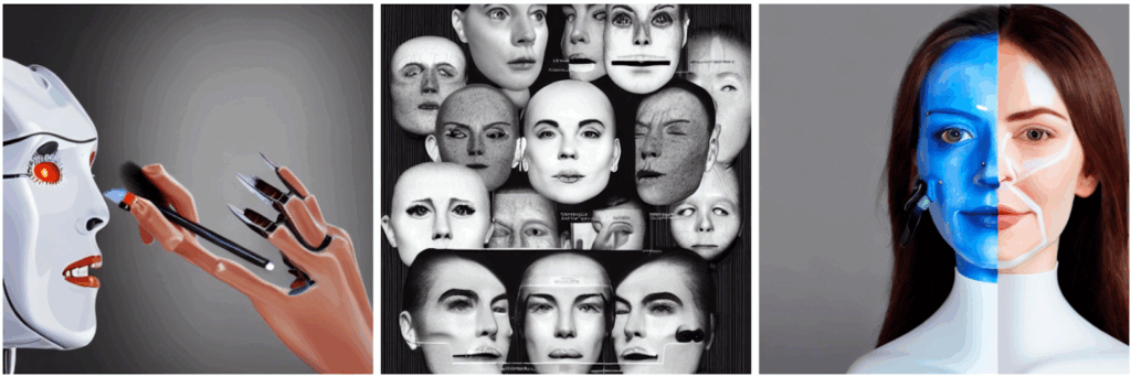
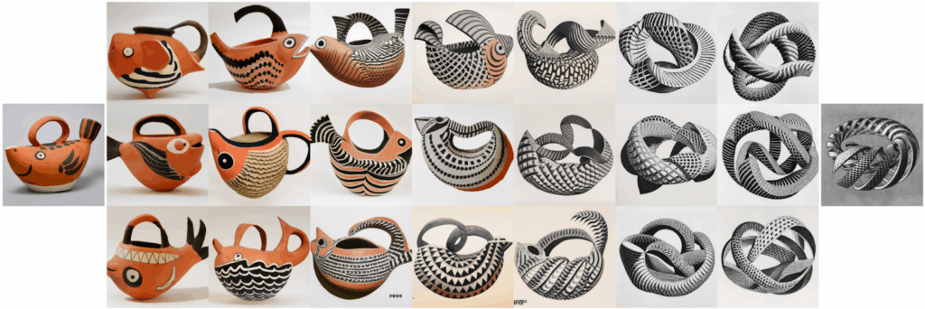
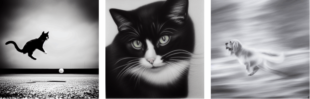
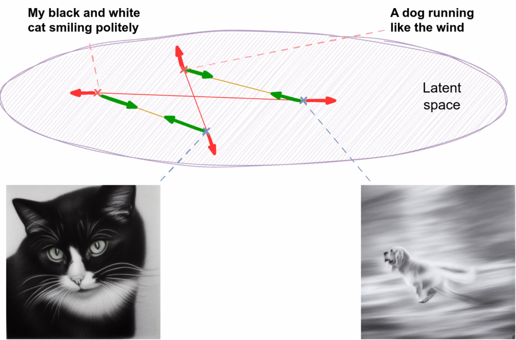
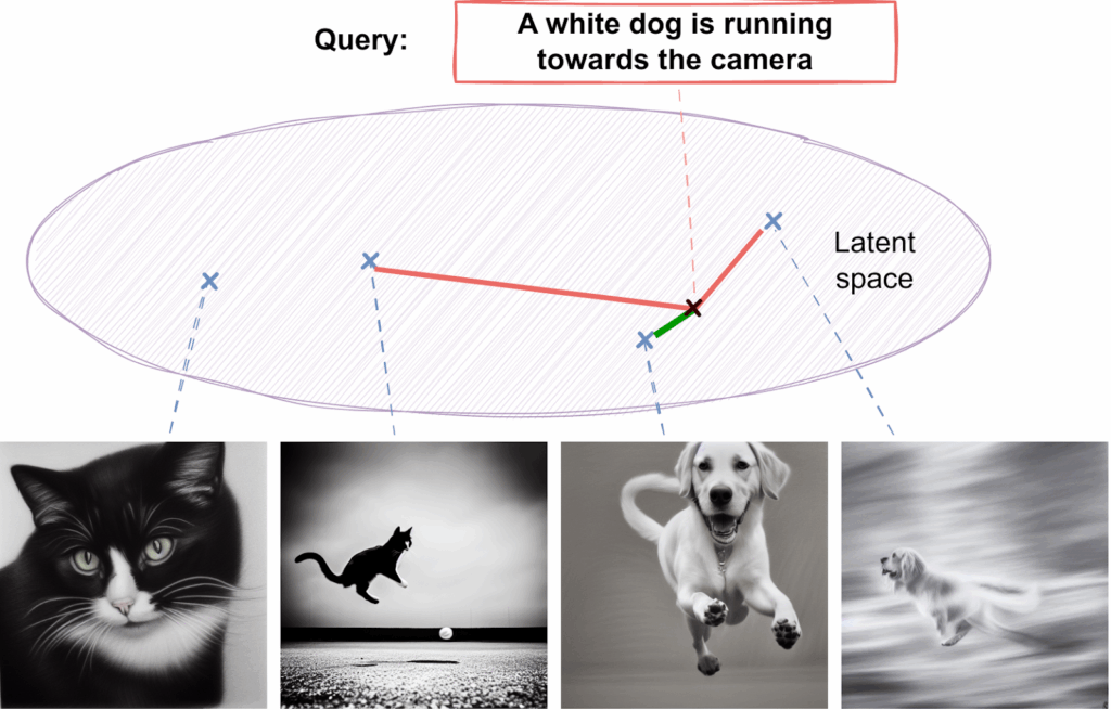
The combination of CLIP embeddings and a diffusion model in the latent space allows DALL-E 2 to do interesting stuff in the latent space. This includes highly semantic interpolations such as this one:
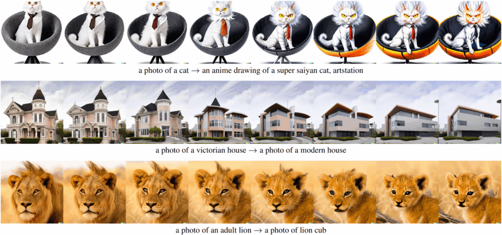
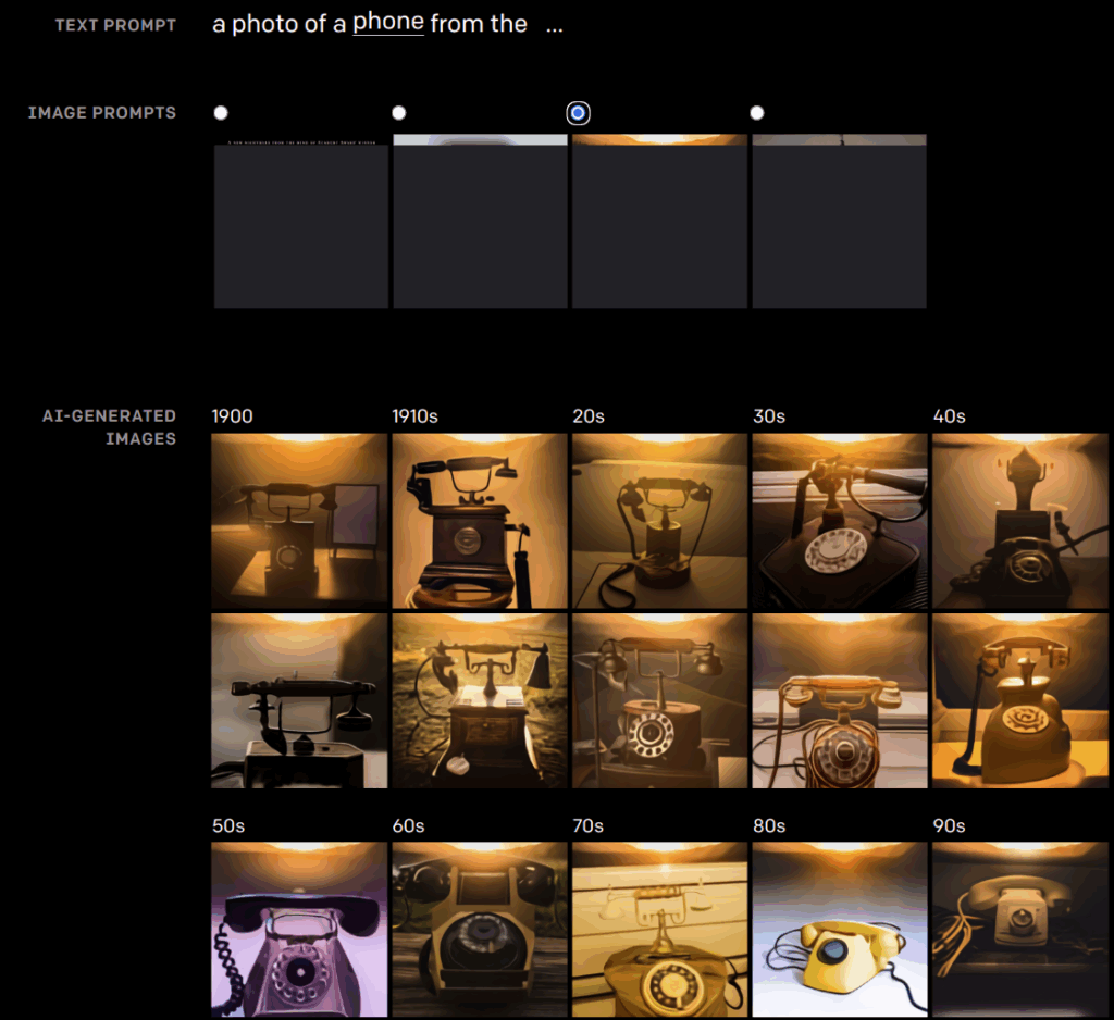
What’s even more interesting, DALL-E 2 can do text-guided image manipulation, changing the image embedding according to the difference between vectors of the original and modified text captions:
DALL-E 2 is not open sourced like Stable Diffusion, and you can only try it via the OpenAI interface. However, at least we have a paper that describes what DALL-E 2 does and how it has been trained (although the paper does appear to gloss over some important details). In the next section, we will not have even that.
Midjourney and controversies over AI-generated art
So what about the elephant in the room? Over the last year, the default models for text-image generation have been neither Stable Diffusion nor DALL-E 2; the lion’s share of the market has been occupied by Midjourney. Unfortunately, there is little I can add to the story above: Midjourney is definitely a diffusion-based model but the team has not published any papers or code, so technical details remain a secret.
The best I could find was this Reddit comment. It claims that the original releases of Midjourney used a diffusion model augmented with progressive distillation (Salimans, Ho, 2022), a process that gradually combines short sampling steps into new, larger sampling steps by learning new samplers:
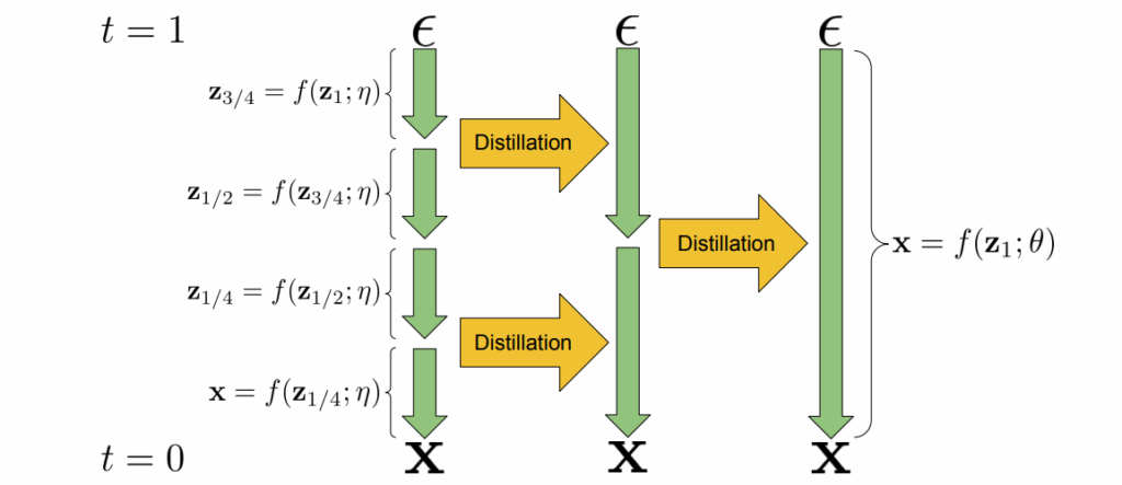
This approach can significantly speed up the sampling process in diffusion models, which we noted as an important problem in the previous post. However, this is just a Reddit comment, and its author admits that available information only relates to the original beta releases, so by now Midjourney models may be entirely different. Thus, in this section let us review the public milestones of Midjourney and the controversies that keep arising over AI-generated art.
One of Midjourney’s first claims to fame was an image called “Théâtre d’Opéra Spatial” (“Space Opera Theatre”) produced by Jason Allen:
This image won first place in a digital art competition (2022 Colorado State Fair, to be precise). Allen signed this work as “Jason M. Allen via Midjourney” and insisted that he did not break any rules of the competition, but the judges were unaware that the image had been AI-generated, so some controversy still ensued.
Later in 2022, Midjourney was used to illustrate a children’s book called “Alice and Sparkle“, very appropriately devoted to a girl who creates a self-aware artificial intelligence but somehow manages to solve the AI alignment problem so in the book, Alice and Sparkle live happily ever after:
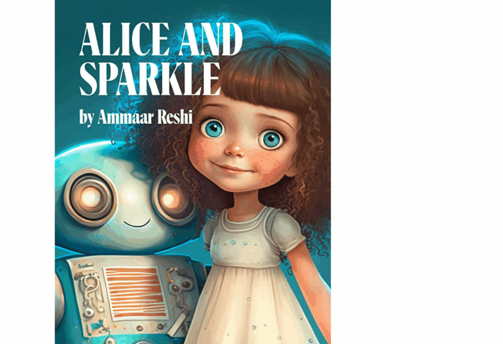
The text of the book was written with heavy help from ChatGPT, and the entire book went from idea to Amazon in 72 hours. It sparked one of the first serious controversies over the legal status of AI-generated art. “Alice and Sparkle” received many 5-star reviews and no fewer 1-star reviews, was temporarily suspended on Amazon (but then returned, here it is), and while there is no legal reason to take down “Alice and Sparkle” right now, the controversy still has not been resolved.
Legal reasons may appear, however. After “Alice and Sparkle”, human artists realized that the models trained on their collective output can seriously put them out of their jobs. They claimed that AI-generated art should be considered derivative, and authors of the art comprising the training set should be compensated. On January 13, 2023, three artists filed a lawsuit against Stability AI, Midjourney, and DeviantArt, claiming that training the models on original work without consent of its authors constitutes copyright infringement. The lawsuit is proceeding as lawsuits generally do, that is, very slowly. In April, Stability AI motioned to dismiss the case since the plaintiffs failed to identify “a single act of direct infringement, let alone any output that is substantially similar to the plaintiffs’ artwork”. On July 23, Judge William Orrick ruled that the plaintiffs did not present sufficient evidence but allowed them to present additional facts to amend their complaint. We will see how the case unfolds, but I have no doubt that this is just the first of many similar cases, and the legal and copyright system will have to adapt to the new reality of generative AI.
In general, over 2023 Midjourney has remained the leader in the AI-generated art space, with several new versions released to wide acclaim. This acclaim, however, has also been controversial: users are often divided over whether new versions of image generation models are actually improvements.
Lately, generated images tend to make the news not as art objects but as fake photographs. AI-generated art has become good enough to pass for real photos, and people have been using it to various effects. In March, Midjourney generated a viral image of Donald Trump being forcefully arrested. On May 22, a Twitter account made to look like a verified Bloomberg feed published a fake image of an explosion near the Pentagon in Washington D.C. The result exceeded expectations: trading bots and/or real traders took the fake news at face value, resulting in a $500B market cap swing:
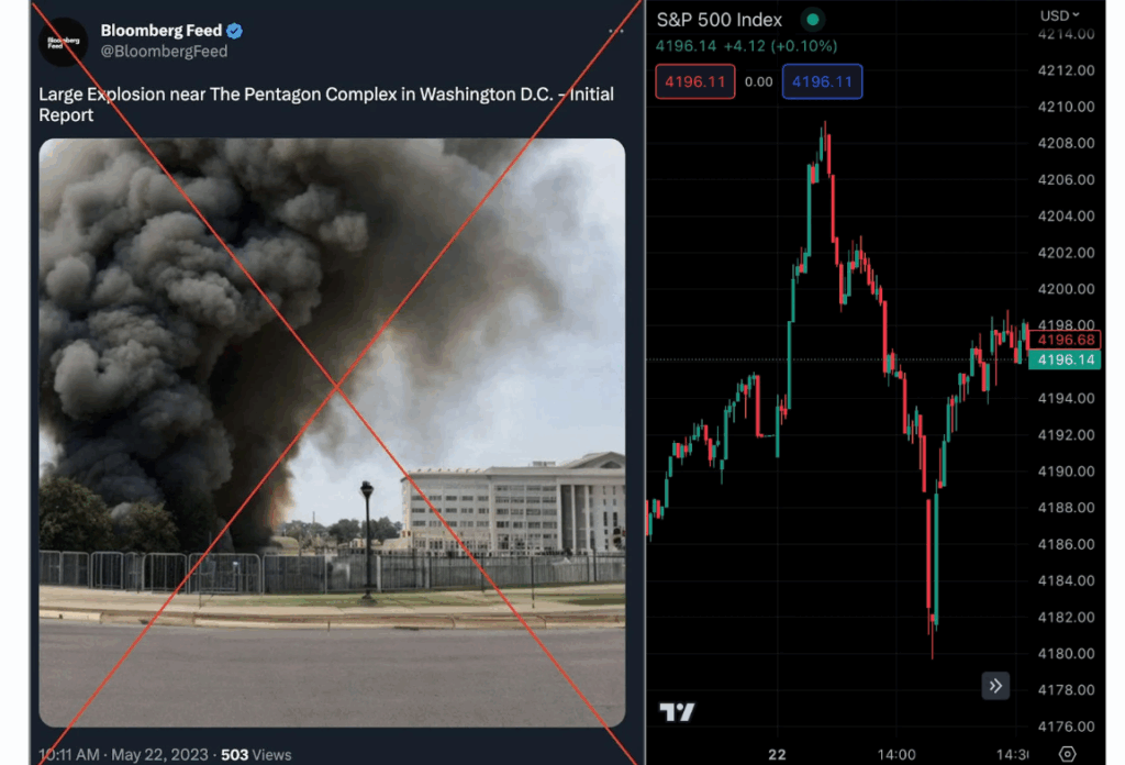
While this kind of news keeps attracting attention to generative AI, to be honest I do not really see a big new issue behind these “deepfakes.” Realistic fake photos have been possible to produce for decades, with the tools steadily improving even regardless of machine learning progress. A Photoshop expert could probably make the Pentagon explosion “photo” in a couple of hours; I am not even sure that fiddling with the prompts to get an interesting and realistic result takes significantly less time (but yes, it does not require an experienced artist). While generative models can scale this activity up, it is by no means a new problem.
Professional artists, on the other hand, face a genuine challenge. I have been illustrating this series of posts with (a rather old version of) Stable Diffusion. In this case, it would not make sense to hire a professional illustrator to make pictures for this blog anyway, so having access to a generative model has been a strict improvement for this series. As long as you are not too scrupulous about the little details, the cats just draw themselves:
But what if I had to illustrate a whole book? Right now, the choice is between spending money to get better quality human-made illustrations and using generative AI to get (somewhat) worse illustrations for free or for a small fee for a Midjourney subscription. For me (the author), the work involved is virtually the same since I would have to explain what I need to a human illustrator as well, and would probably have to make a few iterations. For the publisher, hiring a human freelancer is a lot of extra work and expense. Even at present, I already see both myself and publishing houses choosing the cheaper and easier option. Guess what happens when this option ceases to be worse in any noticeable way…
Conclusion
With this, we are done with the original plan for the “Generative AI” series. Over these seven posts, we have seen a general overview of modern approaches to image generation, starting from the original construction of variational autoencoders and proceeding all the way to the latest and greatest diffusion-based models.
However, a lot has happened in the generative AI space even as I have been writing this series! In my lectures, I call 2023 “the spring of artificial intelligence”: starting from the growing popularity of ChatGPT and the release of LLaMA that put large language models in the hands of the public, important advances have been made virtually every week. So next time, I will attempt to review what has been happening this year in AI; it will not be technical at all but the developments seem to be too important to miss. See you then!
Sergey Nikolenko
Head of AI, Synthesis AI

 , where
  is the input image and
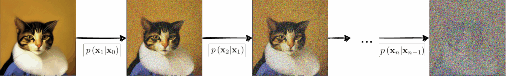
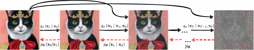
  is the image with added noise. Applying this distribution repeatedly, we get a Markov chain called forward diffusion that gradually adds noise until the image is completely unrecognizable:
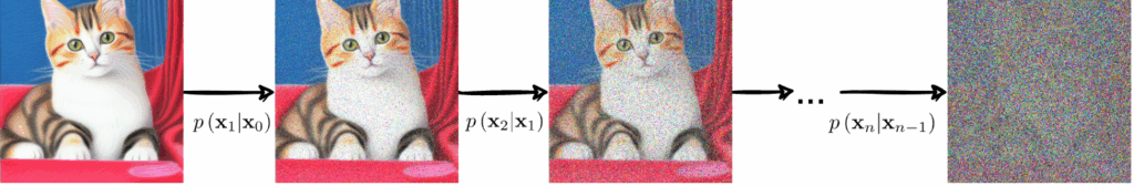
 with model parameters
  that should be a good approximation for the inverted
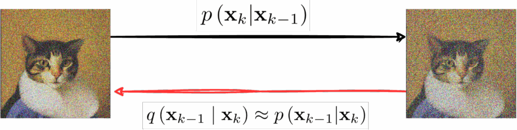
  , you can presumably run it backwards and get the images back from basically random noise. This process is known as reverse diffusion:
 to
to  . Since we already know
  is a Gaussian with variance
  and mean that reduces
  by a factor of the square root of
  (this is necessary to make the process variance preserving, so that
  would not explode or vanish), and the entire process takes T steps:
![\[q(\mathbf{x}_t | \mathbf{x}_{t-1}) = \mathcal{N}\left(\mathbf{x}_t | \sqrt{1-\beta_t}\mathbf{x}_{t-1}, \beta_t\mathbf{I}\right),\qquad q\left(\mathbf{x}_{1:T} | \mathbf{x}_0\right) = \prod_{t=1}^T q\left(\mathbf{x}_t | \mathbf{x}_{t-1}\right).\]](https://blog.sergeynikolenko.ru/wp-content/ql-cache/quicklatex.com-3f2b1e0a2aa9e1fc77fd89d9176d97ed_l3.svg "Rendered by QuickLaTeX.com")

 is also a Gaussian, and we know its parameters:
![\[q\left(\mathbf{x}_{t} | \mathbf{x}_0\right) = \mathcal{N}\left(\mathbf{x}_{t} | \sqrt{A_t}\mathbf{x}_0, \left(1-A_t\right)\mathbf{I}\right).\]](https://blog.sergeynikolenko.ru/wp-content/ql-cache/quicklatex.com-42a7387facdf0eee73c05da98615c98a_l3.svg "Rendered by QuickLaTeX.com")
 directly, in closed form, without having to go through any intermediate steps.
 , it would be easy! Let’s use the Bayes formula and substitute distributions that we already know:

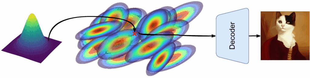
 that represents the impossibly messy distribution of, say, real life images. Ultimately we want our reverse diffusion process to reconstruct
  ; something like this:
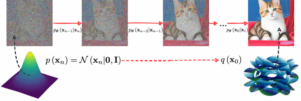
 , with no conditioning on the unknown
 :
:
![\[\log p_{\boldsymbol{\theta}}(\mathbf{x}_0) = \log p_{\boldsymbol{\theta}}(\mathbf{x}_0,\mathbf{x}_1,\ldots,\mathbf{x}_T) - \log p_{\boldsymbol{\theta}}(\mathbf{x}_1,\ldots,\mathbf{x}_T|\mathbf{x}_0),\]](https://blog.sergeynikolenko.ru/wp-content/ql-cache/quicklatex.com-9b929bc3f16ece335bb0fe3af038534e_l3.svg "Rendered by QuickLaTeX.com")
 , and then add and subtract
  on the right-hand side:
![\begin{align*}\mathbb{E}_{q(\mathbf{x}_{0})}\left[\log p_{\boldsymbol{\theta}}(\mathbf{x}_0)\right] &= \mathbb{E}_{q(\mathbf{x}_{0:T})}\left[\log p_{\boldsymbol{\theta}}(\mathbf{x}_{0:T})\right] - \mathbb{E}_{q(\mathbf{x}_{0:T})}\left[\log p_{\boldsymbol{\theta}}(\mathbf{x}_{1:T}|\mathbf{x}_0)\right] \\ & = \mathbb{E}_{q(\mathbf{x}_{0:T})}\left[\log\frac{p_{\boldsymbol{\theta}}(\mathbf{x}_{0:T})}{q(\mathbf{x}_{1:T}|\mathbf{x}_{0})}\right] + \mathbb{E}_{q(\mathbf{x}_{0:T})}\left[\log\frac{q(\mathbf{x}_{1:T}|\mathbf{x}_{0})}{p_{\boldsymbol{\theta}}(\mathbf{x}_{1:T}|\mathbf{x}_{0})}\right].\end{align*}](https://blog.sergeynikolenko.ru/wp-content/ql-cache/quicklatex.com-889edd5ef0cc407f9373b90208aad17c_l3.svg "Rendered by QuickLaTeX.com")
 and
and  , so that’s what we want to minimize in the approximation. Since on the left-hand side we have a constant independent of
  minimizing the KL divergence with respect to
 ![\begin{align*}\mathcal{L} =& \mathbb{E}_{q}\left[\log\frac{q(\mathbf{x}_{1:T}|\mathbf{x}_{0})}{p_{\boldsymbol{\theta}}(\mathbf{x}_{0:T})}\right] = \mathbb{E}_{q}\left[\log\frac{\prod_{t=1}^Tq(\mathbf{x}_{t}|\mathbf{x}_{t-1})}{p_{\boldsymbol{\theta}}(\mathbf{x}_{T})\prod_{t=1}^Tp_{\boldsymbol{\theta}}(\mathbf{x}_{t-1}|\mathbf{x}_{t})}\right] \\=& \mathbb{E}_{q}\left[-\log p_{\boldsymbol{\theta}}(\mathbf{x}_{T}) + \sum_{t=1}^T\log\frac{q(\mathbf{x}_{t}|\mathbf{x}_{t-1})}{p_{\boldsymbol{\theta}}(\mathbf{x}_{t-1}|\mathbf{x}_{t})}\right] \\=& \mathbb{E}_{q}\left[-\log p_{\boldsymbol{\theta}}(\mathbf{x}_{T}) + \sum_{t=2}^T\log\frac{q(\mathbf{x}_{t}|\mathbf{x}_{t-1})}{p_{\boldsymbol{\theta}}(\mathbf{x}_{t-1}|\mathbf{x}_{t})} + \log\frac{q(\mathbf{x}_{1}|\mathbf{x}_{0})}{p_{\boldsymbol{\theta}}(\mathbf{x}_{0}|\mathbf{x}_{1})}\right] \\=& \mathbb{E}_{q}\left[-\log p_{\boldsymbol{\theta}}(\mathbf{x}_{T}) + \sum_{t=2}^T\log\left(\frac{q(\mathbf{x}_{t}|\mathbf{x}_{t-1},\mathbf{x}_{0})}{p_{\boldsymbol{\theta}}(\mathbf{x}_{t-1}|\mathbf{x}_{t})}\frac{q(\mathbf{x}_{t}|\mathbf{x}_{0})}{q(\mathbf{x}_{t-1}|\mathbf{x}_{0})}\right) + \log\frac{q(\mathbf{x}_{1}|\mathbf{x}_{0})}{p_{\boldsymbol{\theta}}(\mathbf{x}_{0}|\mathbf{x}_{1})}\right] \\=& \mathbb{E}_{q}\left[-\log p_{\boldsymbol{\theta}}(\mathbf{x}_{T}) + \sum_{t=2}^T\log\frac{q(\mathbf{x}_{t}|\mathbf{x}_{t-1},\mathbf{x}_{0})}{p_{\boldsymbol{\theta}}(\mathbf{x}_{t-1}|\mathbf{x}_{t})} + \log\frac{q(\mathbf{x}_{T}|\mathbf{x}_{0})}{q(\mathbf{x}_{1}|\mathbf{x}_{0})} + \log\frac{q(\mathbf{x}_{1}|\mathbf{x}_{0})}{p_{\boldsymbol{\theta}}(\mathbf{x}_{0}|\mathbf{x}_{1})}\right] \\=& \mathbb{E}_{q}\left[\log\frac{q(\mathbf{x}_{T}|\mathbf{x}_{0})}{p_{\boldsymbol{\theta}}(\mathbf{x}_{T})} + \sum_{t=2}^T\log\frac{q(\mathbf{x}_{t}|\mathbf{x}_{t-1},\mathbf{x}_{0})}{p_{\boldsymbol{\theta}}(\mathbf{x}_{t-1}|\mathbf{x}_{t})} - \log p_{\boldsymbol{\theta}}(\mathbf{x}_{0}|\mathbf{x}_{1})\right].\end{align*}](https://blog.sergeynikolenko.ru/wp-content/ql-cache/quicklatex.com-d46af7a77afb461be4768ab2ceb638a4_l3.svg "Rendered by QuickLaTeX.com")
 components, and almost all of them are actually KL divergences between Gaussians:
 we are using the Gaussian parametrization
![\[p_{\boldsymbol{\theta}}(\mathbf{x}_{t-1} | \mathbf{x}_t) = \mathcal{N}\left(\mathbf{x}_{t-1}| \boldsymbol{\mu}_{\boldsymbol{\theta}}\left(\mathbf{x}_t,t\right),\Sigma_{\boldsymbol{\theta}}\left(\mathbf{x}_t, t\right)\right)\]](https://blog.sergeynikolenko.ru/wp-content/ql-cache/quicklatex.com-b38ecea4ac4e0118d8ef3bf62ee6ee1d_l3.svg "Rendered by QuickLaTeX.com")
 . For the mean, for instance, we get
![\[\boldsymbol{\mu}_{\boldsymbol{\theta}}\left(\mathbf{x}_t,t\right) \approx {\tilde{\boldsymbol{\mu}}}_t\left(\mathbf{x}_t,\mathbf{x}_0\right) = \frac{1}{\sqrt{A_t}}\left(\mathbf{x}_t - \frac{1-\alpha_t}{\sqrt{1-A_t}}\boldsymbol{\epsilon}_t\right),\]](https://blog.sergeynikolenko.ru/wp-content/ql-cache/quicklatex.com-41638ba4e70a29ad82ee7804ea6c1fa0_l3.svg "Rendered by QuickLaTeX.com")
 during training, we can actually parametrize the noise directly rather than the mean:
![\[p_{\boldsymbol{\theta}}(\mathbf{x}_{t-1} | \mathbf{x}_t) = \mathcal{N}\left(\mathbf{x}_{t-1}\middle| \frac{1}{\sqrt{\alpha_t}}\left(\mathbf{x}_t-\frac{1-\alpha_t}{\sqrt{1-A_t}}\boldsymbol{\epsilon}_{\boldsymbol{\theta}}\left(\mathbf{x}_t,t)\right),\Sigma_{\boldsymbol{\theta}}(\mathbf{x}_t, t\right)\right).\]](https://blog.sergeynikolenko.ru/wp-content/ql-cache/quicklatex.com-b70510b46329a9dbb6794846d36adce9_l3.svg "Rendered by QuickLaTeX.com")
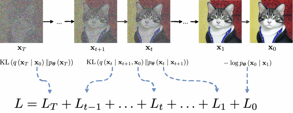
 ; since
  is a fixed distribution that we want to sample from, this means that LT is a constant and can be ignored;
 either, setting them to
  for some constant
  ; they also develop the noise reparametrization mentioned above somewhat further, obtaining a simple closed form for
  ; namely, they assume that the data consists of integers from 0 to 255 scaled linearly to [-1, 1], which is a natural representation for images, and model
![\[p_{\boldsymbol{\theta}}(\mathbf{x}_{0} | \mathbf{x}_1) = \prod_{i=1}^D\int_{\delta_-\left({x}_0,i\right)}^{\delta_+\left({x}_0,i\right)} \mathcal{N}\left({x}\middle|{\mu}_{\boldsymbol{\theta},i}\left(\mathbf{x}_1\right), \sigma_1^2\right)\mathrm{d} x,\]](https://blog.sergeynikolenko.ru/wp-content/ql-cache/quicklatex.com-c92b31f1e22e0e69bfe494d902e9e69b_l3.svg "Rendered by QuickLaTeX.com")
 goes over the pixels (components of
  ),
),  is the independent decoder model, and the integration limits define an interval of length 1/255 on every side of
  , which is a standard trick to make everything smooth and continuous.
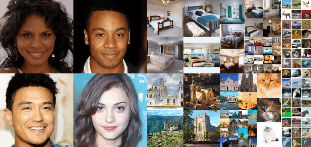
 but only on the marginal distributions
 ![\[q_{\sigma}\left(\mathbf{x}_{1:T} | \mathbf{x}_0\right)= q_{\sigma}\left(\mathbf{x}_{T} | \mathbf{x}_0\right)\prod_{t=2}^T q_{\sigma}\left(\mathbf{x}_{t-1} | \mathbf{x}_{t},\mathbf{x}_0\right).\]](https://blog.sergeynikolenko.ru/wp-content/ql-cache/quicklatex.com-482a6dc2586418ffb010e709109ee38c_l3.svg "Rendered by QuickLaTeX.com")
![\[q_{\sigma}\left(\mathbf{x}_{t} | \mathbf{x}_{t-1},\mathbf{x}_0\right)=\frac{q_{\sigma}\left(\mathbf{x}_{t-1} | \mathbf{x}_{t},\mathbf{x}_0\right)q_{\sigma}\left(\mathbf{x}_{t} | \mathbf{x}_0\right)}{q_{\sigma}\left(\mathbf{x}_{t-1} | \mathbf{x}_0\right)}.\]](https://blog.sergeynikolenko.ru/wp-content/ql-cache/quicklatex.com-3be2d15e4762b401aefac0467145311b_l3.svg "Rendered by QuickLaTeX.com")
 that gets us from
  , we are now approximating the random noise
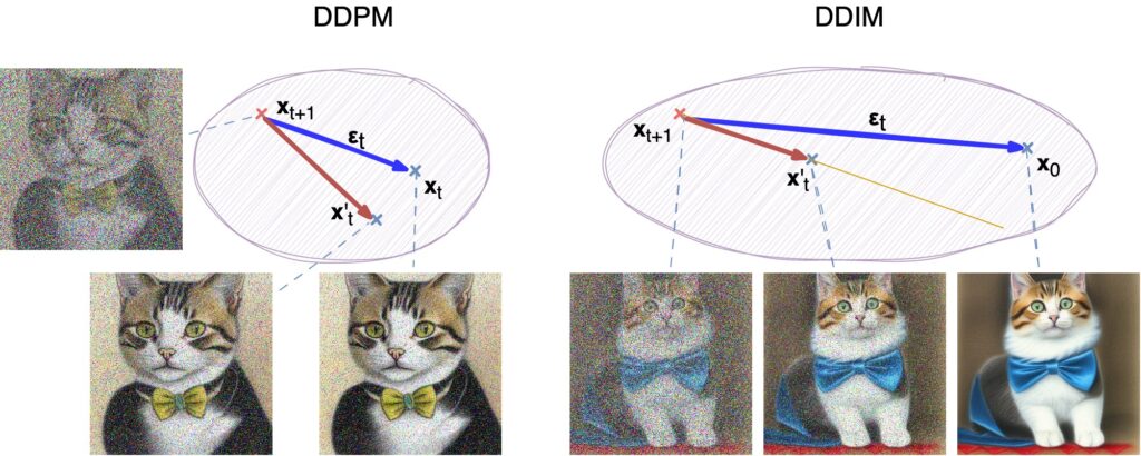
 and the dependence on
  in a single step with correspondingly increased
  ! One can train a model with a large number of steps
  but sample only a few of them in the generation part, which speeds things up very significantly. Naturally, the variance will increase, and the approximations will get worse, but with careful tuning this effect can be contained.
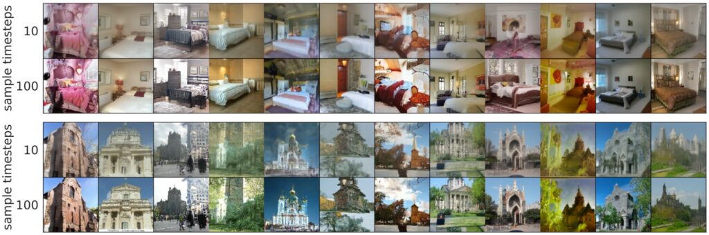
 corresponds to exactly one image, and now we can expect DDIMs to behave in the same way as other models that train latent representations (compare, e.g.,
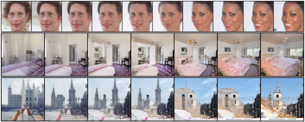
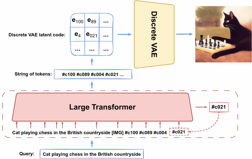
![\[p_{\mathbf{\theta},\mathbf{\psi}}(\mathbf{x},\mathbf{y},\mathbf{z})= p_{\mathbf{\theta}}(\mathbf{x} | \mathbf{y},\mathbf{z})p_{\mathbf{\psi}}(\mathbf{y},\mathbf{z}),\]](https://blog.sergeynikolenko.ru/wp-content/ql-cache/quicklatex.com-665f2cf6c3eb2e073ded3b63cb8692c1_l3.svg "Rendered by QuickLaTeX.com")
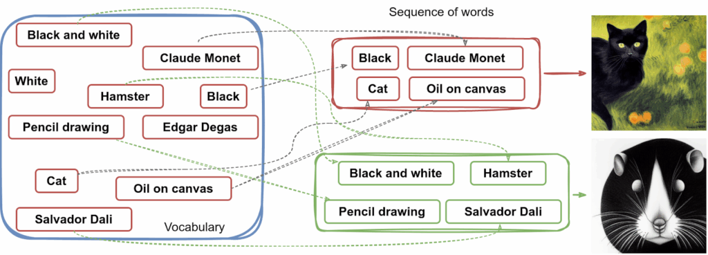
 is the corresponding text description, and
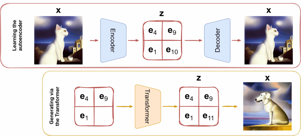
  is the image’s latent code. The Transformer learns to generate
  since it inevitably becomes a generative model for text as well), and the result is used by the discrete VAE, so actually we assume that
  .
.![\[\log p_{\mathbf{\theta},\mathbf{\psi}}(\mathbf{x},\mathbf{y}) \ge \mathbb{E}_{\mathbf{z}\sim q_{\mathbf{\phi}}(\mathbf{z}|\mathbf{x})}\left[ \log p_{\mathbf{\theta}}(\mathbf{x}|\mathbf{y},\mathbf{z}) - \beta\mathrm{KL}\left(q_{\mathbf{\phi}}(\mathbf{z}|\mathbf{x})\| p_{\mathbf{\psi}}(\mathbf{y},\mathbf{z})\right)\right],\]](https://blog.sergeynikolenko.ru/wp-content/ql-cache/quicklatex.com-2c082d6cffd253767b8fe67c9afe5543_l3.svg "Rendered by QuickLaTeX.com")
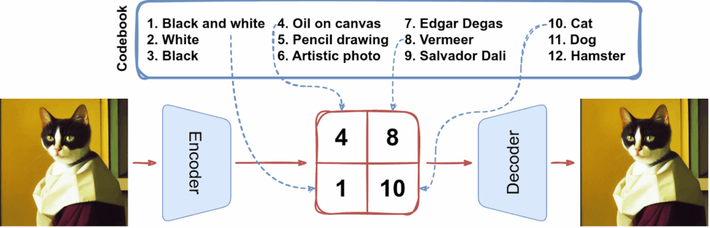
 is the distribution of latent codes produced by the discrete VAE’s encoder from an image
  here denotes the parameters of the discrete VAE’s encoder;
 is the distribution of images generated by the discrete VAE’s decoder from a latent code
  ;
;  stands for the parameters of the discrete VAE’s decoder;
 is the joint distribution of texts and latent codes modeled by the Transformer; here
  denotes the Transformer’s parameters.
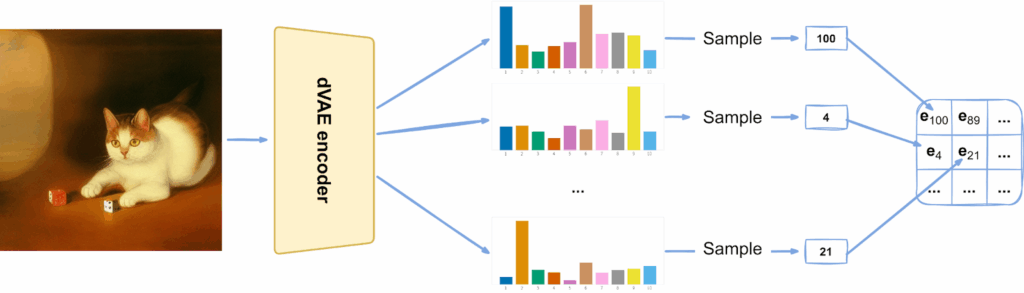
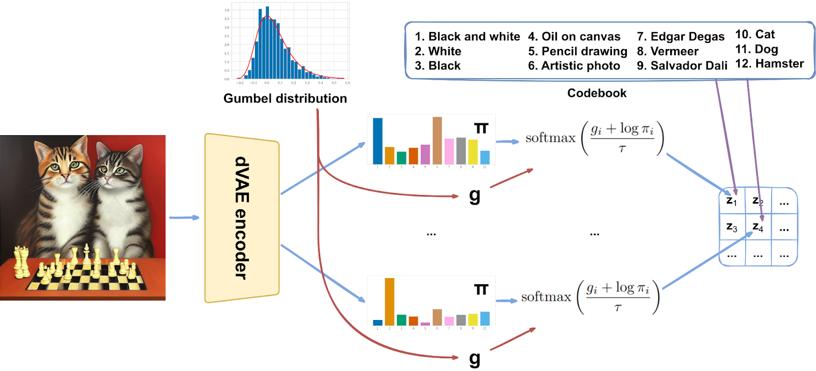
![\[p(g_i) = e^{-\left(g_i + e^{-g_i}\right)},\qquad F(g_i) = e^{-e^{-g_i}}.\]](https://blog.sergeynikolenko.ru/wp-content/ql-cache/quicklatex.com-ba07122ecf12ce18a54348e8eafb06cb_l3.svg "Rendered by QuickLaTeX.com")
![\[z = \arg\,\max_i\left(g_i + \log \pi_i\right).\]](https://blog.sergeynikolenko.ru/wp-content/ql-cache/quicklatex.com-b3f540bcd93d3c6200b013a4585fbfd8_l3.svg "Rendered by QuickLaTeX.com")
![\[y_i = \mathrm{softmax}\left(\frac{1}{\tau}\left(g_i + \log\pi_i\right)\right) = \frac{e^{\frac{1}{\tau}\left(g_i + \log\pi_i\right)}}{\sum_je^{\frac{1}{\tau}\left(g_j + \log\pi_j\right)}}.\]](https://blog.sergeynikolenko.ru/wp-content/ql-cache/quicklatex.com-b62c83de2e58b80c4380e05f88d0c6db_l3.svg "Rendered by QuickLaTeX.com")
 this tends to a discrete distribution with probabilities
  , and during training we can gradually reduce the temperature τ. Note that now the result is not a single codebook vector but a linear combination of codebook vectors with weights
  .
.
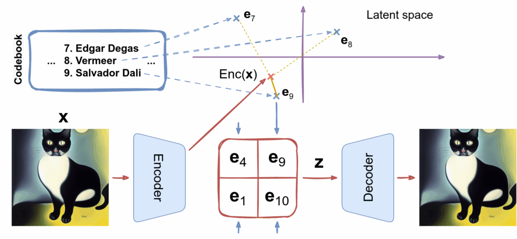
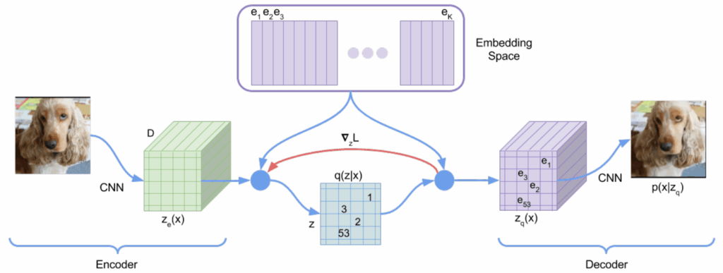
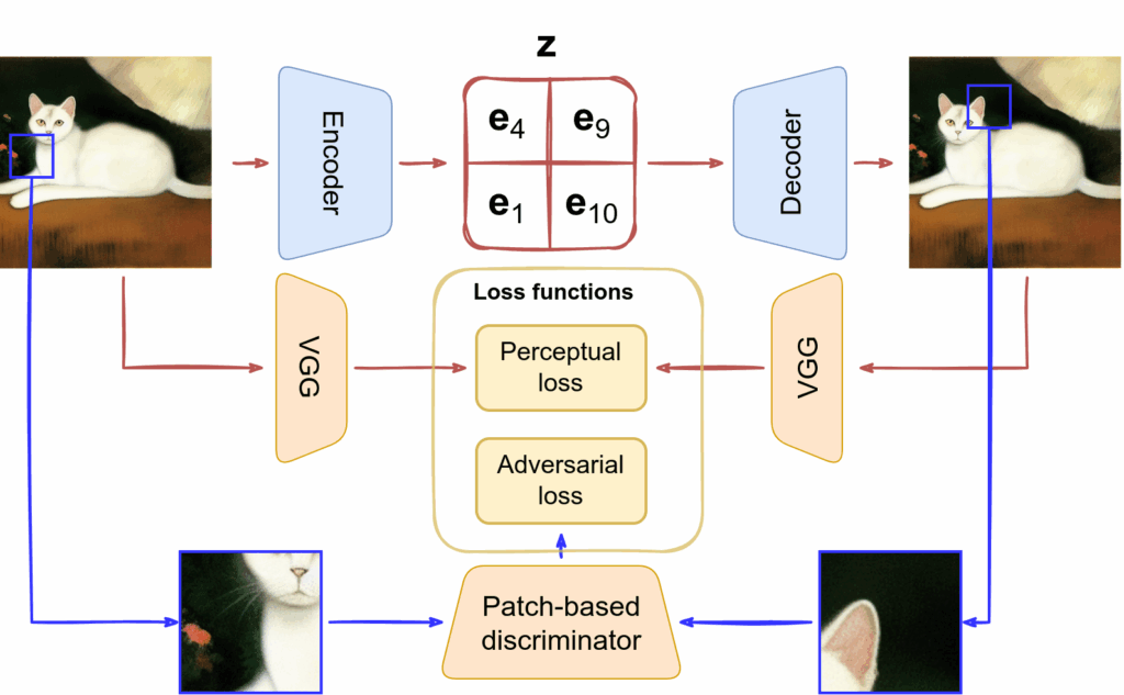
![\[\mathcal{L} = -\log p(\mathbf{x}|\mathbf{z}_q(\mathbf{x}) + \left\|\mathrm{sg}\left[\mathbf{z}_e(\mathbf{x})\right]-\mathbf{e}\right\|_2^2 + \beta\left\|\mathbf{z}_e(\mathbf{x}) - \mathrm{sg}\left[\mathbf{e}\right]\right\|_2^2.\]](https://blog.sergeynikolenko.ru/wp-content/ql-cache/quicklatex.com-00894d566cf8b3d8a7d2f321e7a3f8d8_l3.svg "Rendered by QuickLaTeX.com")
 and
and  are two latent representations for an image
  is the output of the decoder and
  is the codebook representation after replacing each vector with its nearest codebook neighbor (this notation is illustrated in the image above); the first term is responsible for training the decoder network;
 is the distribution of reconstructed images after the decoder given the latent code; we want the reconstruction to be good so we maximize the likelihood of the original image
  ) and zero during the backward pass (when we compute the gradient
  );
); closer to the latent codes
  can balance the two terms although the authors say that the results don’t change for
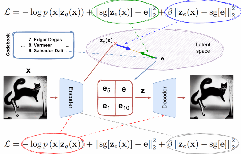

![\[p(\mathbf{z})p(\mathbf{x}|\mathbf{z})=p(\mathbf{x},\mathbf{z})=p(\mathbf{x})p(\mathbf{z}|\mathbf{x})\]](https://blog.sergeynikolenko.ru/wp-content/ql-cache/quicklatex.com-d22a714c241adc27cf598aa1ea0e9c3b_l3.svg "Rendered by QuickLaTeX.com")
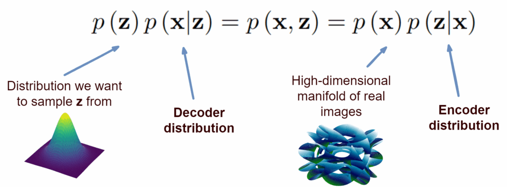
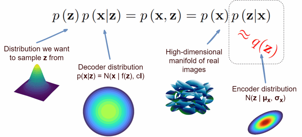
![\[\begin{aligned} p(\mathbf{x},\mathbf{z}) &= p(\mathbf{x})p(\mathbf{z}|\mathbf{x}),\\ \log p(\mathbf{x},\mathbf{z}) &= \log p(\mathbf{x}) + \log p(\mathbf{z}|\mathbf{x}),\\ \log p(\mathbf{x}) &= \log p(\mathbf{x},\mathbf{z}) - \log p(\mathbf{z}|\mathbf{x}),\\\log p(\mathbf{x}) &= \mathbb{E}_{q(\mathbf{z})}\left[\log p(\mathbf{x},\mathbf{z}) - {\log q(\mathbf{z})} + {\log q(\mathbf{z})} - {\log \p(\mathbf{z}|\mathbf{x})\right],\\\log p(\mathbf{x}) &= \int {q(\mathbf{z}}}{\log \frac{p(\mathbf{x},\mathbf{z})}{q(\mathbf{z})}}\dd\mathbf{z} + \int {q(\mathbf{z})}{\log \frac{q(\mathbf{z})}{p(\mathbf{z}|\mathbf{x})}\mathrm{d}\mathbf{z}. \end{aligned}\]](https://blog.sergeynikolenko.ru/wp-content/ql-cache/quicklatex.com-3eace644227b76ee22fff22f10fbbeda_l3.svg "Rendered by QuickLaTeX.com")
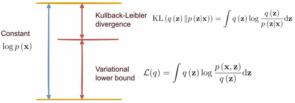
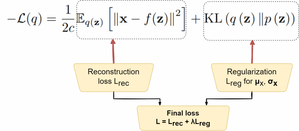
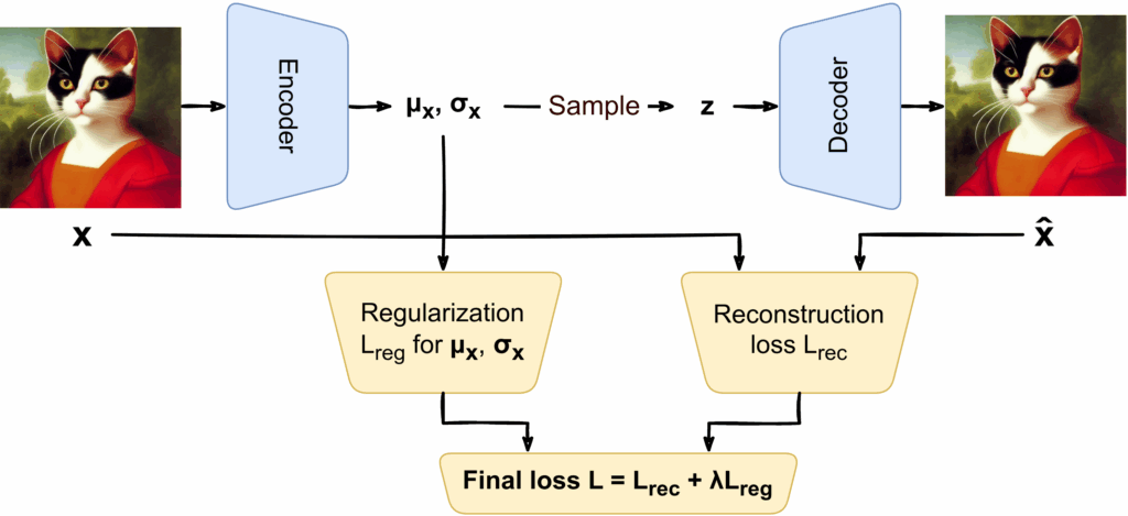
![\[\begin{aligned}\mathcal{L}(q) &= \int {q(\mathbf{z})}{\log \frac{p(\mathbf{x},\mathbf{z})}{q(\mathbf{z})}}\mathrm{d}\mathbf{z} = \int {q(\mathbf{z})}{\log \frac{p(\mathfb{z})p(\mathbf{x}|\mathbf{z})}{q(\mathbf{z})}}\mathrm{d}\mathbf{z} \\&= \int {q(\mathbf{z})}{\log {p(\mathbf{x}|\mathbf{z})}}\mathrm{d}\mathbf{z} + \int {q(\mathbf{z})}{\log \frac{p(\mathbf{z})}{q(\mathbf{z})}}\mathrm{d}\mathbf{z} \\&= \int {q(\mathbf{z})}{\log \mathcal{N}(\mathbf{x}| f(\mathbf{z}),c\mathbf{I})}\mathrm{d}\mathbf{z} - \kl{q(\mathbf{z})}{p(\mathbf{z})} \\&= -\frac{1}{2c}\mathbb{E}_{q(\mathbf{z})}\left[ \left|\mathbf{x} - f(\mathbf{z})\right|^2\right] - \mathrm{KL}\left({q(\mathbf{z})}\|{p(\mathbf{z})}\right).\end{aligned}\]](https://blog.sergeynikolenko.ru/wp-content/ql-cache/quicklatex.com-56f44eeb226e6924c96c9f8bd7fa94a8_l3.svg "Rendered by QuickLaTeX.com")
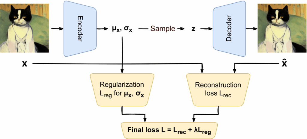
![\[\mathcal{L} = \mathcal{L}_{\mathrm{rec}} + \lambda\mathcal{L}_{\mathrm{reg}}.\]](https://blog.sergeynikolenko.ru/wp-content/ql-cache/quicklatex.com-767324e9e5f9c0db1d8142be37b299bf_l3.svg "Rendered by QuickLaTeX.com")