On May 22–23, Neuromation had the honor of taking part in one of the most interesting interdisciplinary gatherings in computer vision and graphics: the LDV Vision Summit, hosted by the LDV Capital foundation. Members of our team in attendance included CTO Artyom Astafurov, CRO Sergey Nikolenko, Head of Product Matthew Moore, and VP Digital Economy Arthur McCallum.
Neuromation’s Chief Research Officer Sergey Nikolenko participated in a panel titled “Synthetic Media Will Disrupt or Empower Media & Technology Giants” about the role of synthetic data in artificial intelligence. The panel discussed key applications of synthetic data and achieved consensus regarding the growing importance of synthetic data in AI as well as the increasing role that synthetic media will play in the future.
One of the key features of the event was that it was truly cross-disciplinary: our team had the pleasure of meeting professionals from AI startups specializing in computer vision and computer graphics, media companies, news outlets, and investors who saw many promising startups at the event. Neuromation is always happy to visit and support important interdisciplinary events. After all, we can only make the future of AI together. Big thanks to the organizers, in particular Evan Nisselson, LDV General Partner, and Abigail Hunter-Syed, LDV VP of Operations; it was their conference more than anyone else’s.
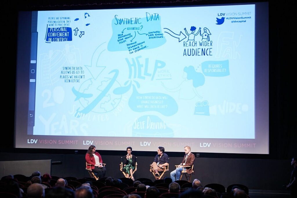
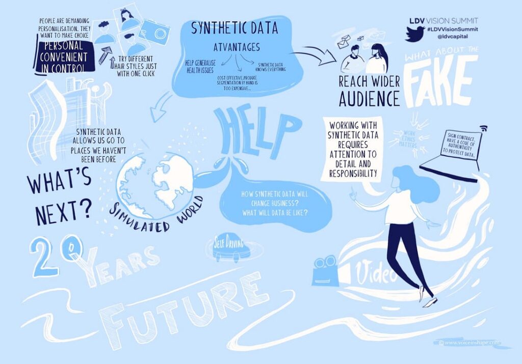
Interestingly, panel discussions at the LDV Vision Summit were accompanied by live illustrations: a hired artist was doodling along as the participants spoke. It looked very cool in the process, and here is what the result looked like for the synthetic data panel.
The list of accepted papers for ICLR 2019 (International Conference on Learning Representations) is already available online, and there are a number of very interesting papers there waiting to be reviewed. So, with the next several posts I thought we could dive into the best of them and discuss some related and very relevant areas.
First off, the work of the renowned AI researcher Dmitry Vetrov. Dmitry has always been, so to speak, a “big brother” in AI for me. I remember how we first met: back in 2009, we made at least two laps around the Moscow State University campus (quite a walk!), talking about machine learning, deep learning, and the future of AI. Or, better to say, Dmitry was talking and I was listening. By now, Dmitry Vetrov is a laboratory leader at the Samsung AI Center Moscow, a research professor and laboratory head at the Higher School of Economics in Moscow, founder and head of the Bayesian Methods Research Group, one of the strongest ML research groups in Russia, and generally one of the most famous ML researchers in Russia. He has always advocated bringing Bayesian methods to deep learning, and many of his works are devoted to exactly this.
ICLR 2019 has become a very successful conference for Dmitry: he (naturally, not alone but with the researchers and students of his labs) has co-authored three papers accepted to ICLR! This is an outstanding achievement, so I decided to take the first NeuroNugget of the “ICLR in Review” series to say thank you to Dmitry Vetrov for all the advice, guidance, and, most importantly, simply a good example he has been setting for all of us through the years. Thank you Dima, and let’s review your latest and greatest!
I shall be telling this with a sigh Somewhere ages and ages hence: Two roads diverged in a wood, and I — I took the one less traveled by, And that has made all the difference.
Robert Frost
Variance Networks: Unexpectedly, Expectation Is Not Required
All of our readers probably know that randomization plays a central role in the training of modern neural networks. There is no way (and no need) to try to replace stochastic gradient descent with a regular one when using randomized mini-batches is orders of magnitude more efficient. Random initialization of the network weights has entirely replaced the unsupervised pre-training methods that jumpstarted the deep learning revolution back in 2006–2007, and new improvements in random initialization methods keep popping up (for example, Xavier initialization for symmetric activation functions, He initialization for ReLU, Le-Jaitly-Hinton for recurrent networks of ReLUs, and many more).
What is a bit less commonly known is that not only is the training randomized, but the networks themselves often are too, as in stochastic neural network constructions where the weights of the network are randomized not just during initialization but throughout training and even during inference as well.
Can you name the most common example of such a construction?..
…[I’ll just give you a little bit of space to think]…
…that’s right, dropout!
A dropout layer makes any network into a stochastic one. Each weight with value w is accessed through a probability distribution, albeit a very simple one. With probability p it’s w, and with probability (1-p) it’s 0. Dropout is very common, so now you see that stochastic neural networks are actually all over the place.
Dropout also showcases another important trick done with stochastic neural networks: weight scaling. In order to do inference with (that is, apply) a stochastic neural network, it might look like you need to run it several times and then average the results, getting an estimate for the resulting expectation which is usually intractable in any other way; this is known as test-time averaging.
But running a network 20 times to get a single answer is not too fast either! Weight scaling is the technique of approximating this process by replacing each weight with its expected value. In the case of dropout, this means that instead of running the network many times for every test example, we replace each weight w subject to dropout with its expected value pw.
Weight scaling is not really formally correct, but is used very widely. As Neklyudov et al. emphasize, its “success… implies that a lot of learned information is concentrated in the expected value of the weights”. But the main point of their paper is to introduce the so-called variance layers: stochastic layers where the expected values carry exactly zero information because the expectations are always set to zero, and only variances of the weights are trained!
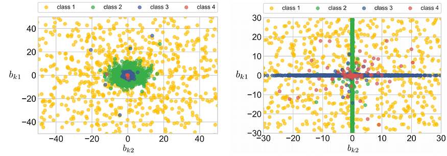
This counterintuitive construction proves to be an interesting one. It turns out that variance layers can and do train and encode interesting features. Here is an illustration for a toy problem:
The two pictures above show two different ways that neurons at a variance layer can interact. On the left, the two neurons encode the four classes together, in almost exactly the same way: class 4 is encoded by the lowest variance (the red core at the origin), class 3 has higher variance, and so on. By using two neurons in the same way, the network can have a whole “sample” of the same underlying distribution, which makes for a more reliable estimate of the variance.
On the right, the two neurons decided to learn complementary things: the first neuron (Y-axis) has high variance for classes 1 and 2, and the second neuron (X-axis) has high variance for classes 1 and 3.
Neklyudov et al. show that variance networks can perform well on standard tasks, they prove to be more robust against adversarial attacks and can improve exploration in reinforcement learning. But most importantly, it turns out that expectations of the weights are not as crucial as people thought. This is a fascinating proof of concept. Who knows, maybe this will lead to a completely new genre of deep learning; we’ll have to wait and see.
The Deep Weight Prior
The second paper co-authored by Dmitry Vetrov at ICLR 2019 is “The Deep Weight Prior” by Andrei Atanov, Arsenii Ashukha, Kirill Struminsky, Dmitry Vetrov, and Max Welling, considers another key element of the Bayesian framework: prior distributions.
Let’s begin with the main formula of all machine learning — Bayes’ rule:
In machine learning, θ usually represents the model parameters, and D represents the data. The formula shows how we change our beliefs about the parameters θ after getting experimental results D: we update our prior belief p(θ) by essentially multiplying it by the likelihood p(D|θ). Recalculating p(θ) into p(D|θ) is the essence of Bayesian inference, and the essence of many machine learning problems and techniques.
But if this is the core of all machine learning, why don’t we hear more about prior distributions in deep learning? The simple answer is that nobody knows how to make nontrivial priors for complex neural networks. Naturally, an L2 regularizer can be thought of as a zero-mean Gaussian prior… but what if we are looking for something more meaningful?
Atanov et al. propose a novel and interesting way to tackle this problem. Specifically, they consider the case of convolutional neural networks, where:
it is very plausible that convolutional layers, especially early ones, learn nearly the same features on all datasets from an entire domain — after all, most modern computer vision networks start out by pretraining on ImageNet even if their goal is not to recognize its classes;
on the other hand, it makes little sense to assume that the prior distribution can decompose into a product over individual weights since the weight matrix of a convolution should represent a single object for this distribution.
Based on these remarks, Atanov et al. rightly assume that they can learn the prior distribution for a convolutional network on other datasets from the same domain (e.g., on smaller datasets of real photographs or handwritten digits), and that this prior distribution, while it factorizes over the layers and channels, will not factorize over the spatial dimensions of the filters, i.e., it will be a distribution over the weight matrices of convolutional filters.
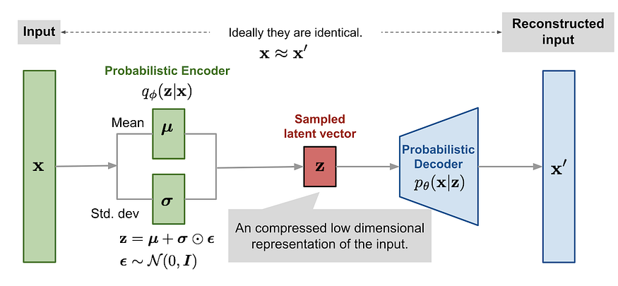
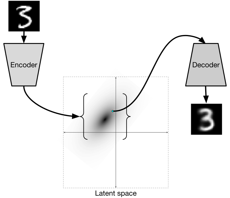
So, how do you train a distribution like that? That’s where variational autoencoders (VAE) come in. We have already discussed VAEs in a previous post. Essentially, they learn a transformation from input x and some random bits with a fixed distribution to a distribution on the latent embeddings q(z|x) that should approximate p(z|x), by learning to output the parameters of q(z|x) (reparametrization trick), and then this distribution on the latent space z can be used through the decoder to make more samples from p(x):
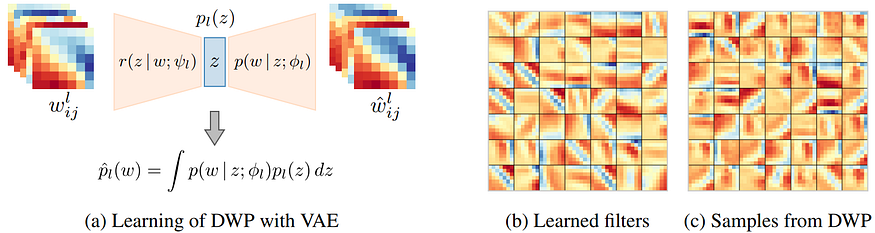
So what do Atanov et al. do? They opt to take some (smaller and simpler) datasets and train a number of convolutional nets (“source networks”) to get a dataset of convolutions. Then they train a VAE on this dataset to produce the prior distribution on the convolutional kernels! This VAE is now a model that can sample from the distribution of convolutional kernels and that defines the deep weight prior:
Then they show that variational inference on the convolutional weights with the deep weight prior works much better than with any other previously known kind of prior. But, again, the most important point here is not a specific experimental result but the idea that it can open up wonderful new possibilities for, among other things, transfer learning and domain adaptation.
Variational Autoencoder with Arbitrary Conditioning
And speaking of variational autoencoders… In the third ICLR paper by Vetrov’s group, “Variational Autoencoder with Arbitrary Conditioning”, Oleg Ivanov, Michael Figurnov, and Dmitry Vetrov introduce a very interesting extension for the VAE framework.
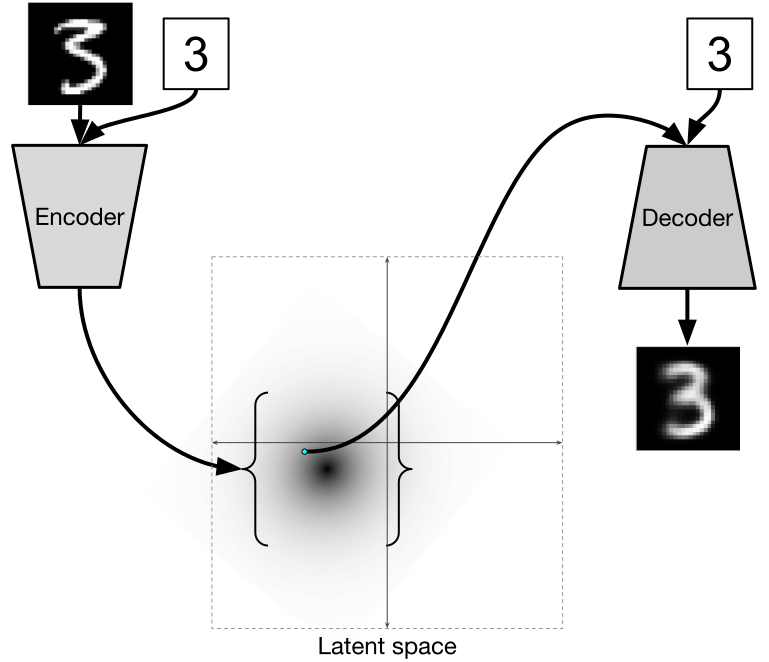
Once you have a generative model (of any kind) and can sample objects from a distribution, the natural next step is to try to construct a conditional version of the same model. This will let you create objects that are subject to some kind of condition; e.g., generate the face of a person with a given age and gender, or with a smile and sunglasses. Traditional conditional VAEs are well-known, of course; to add a label to the VAE construction, you can simply input it to both encoder and decoder, like this:
Now the model is free to learn completely different distributions in the latent space for different labels, and this produces all sorts of wonderful effects, has implications for style transfer, and so on.
In this paper, Ivanov et al. take conditioning up to eleven: they consider a situation where any subset of the input might be unknown and subject to generation conditioned on the available part. That is:
along with the input x, we are given a binary mask b that shows which components (pixels) of x are known (where bi=0) and which are not (where bi=1);
the goal is to construct a model for the conditional distribution p(xb|x1-b,b);
as part of the problem setting, we are also given a prior distribution on the masks p(b) that shows which masks are more likely to appear and which, therefore, the model should concentrate on.
To solve this problem, Ivanov et al. propose a model they call Variational Autoencoder with Arbitrary Conditioning (VAEAC). A full consideration of VAEAC, its training and inference goes, alas, far beyond the scope of a NeuroNugget. But I do want to note the uses of the resulting model. The arbitrary conditioning setting is designed for problems such as:
missing features imputation, i.e., reconstructing missing features in a dataset; in the wild, many datasets are rather dirty, but we cannot afford to simply discard all the incomplete data;
image inpainting, i.e., reconstructing a hidden part of an image; this is an important problem for image manipulation, e.g., if you want to delete a random passerby from your photo, you can segment the person and cut them out with a segmentation model, but then you still need to inpaint the background in a natural way in place of the person.
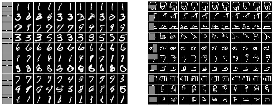
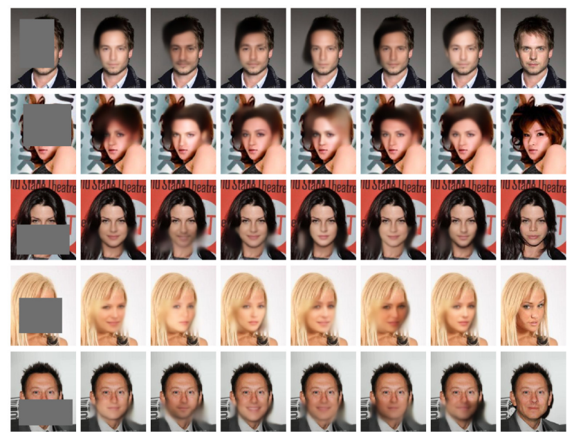
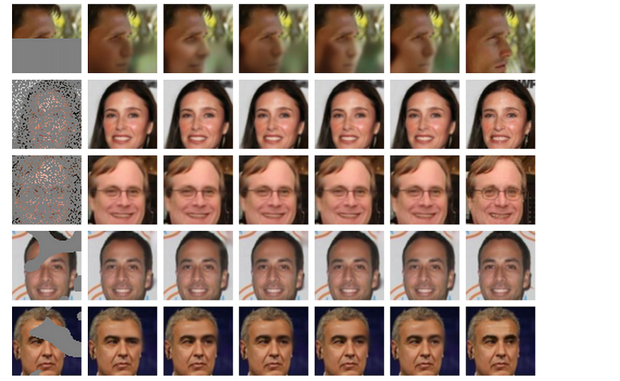
VAEAC solves both of these problems nicely. It especially shines on imputation, but that use-case is not flashy enough, so here are some inpainting results. The rightmost columns in the following images show the ground truth. Top to bottom: MNIST and Omniglot, CelebA, and CelebA with more interesting masks:
Stochastic Weight Averaging: A Simple Trick to Rule Your Networks
But wait, there is more! This is not an ICLR paper yet, but it’s a very recent work from Dmitry’s lab that might prove applicable to nearly everyone in the world of deep learning. In “Averaging Weights Leads to Wider Optima and Better Generalization”, Pavel Izmailov, Dmitrii Podoprikhin, Timur Garipov, Dmitry Vetrov, and Andrew Gordon Wilson present a simple idea that can be embedded into many networks at virtually no cost… but quite possibly with a hefty profit!
It is common knowledge in machine learning that putting together a number of different models, in a procedure known as ensembling, helps improve performance. However, in deep learning ensembling is hard: training even one model is difficult, and getting a hundred meaningful networks together would be quite a computational feat.
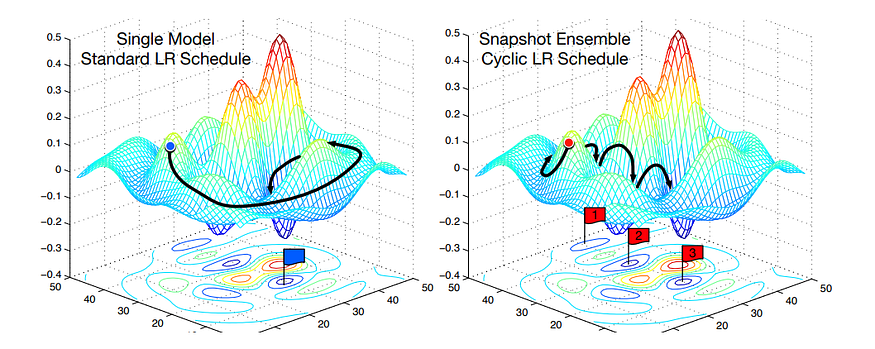
There have been some works on ensembling in deep learning, though. Inspired by the ideas of cyclical learning rates, Huang et al. in “Snapshot Ensembles: Train 1, get M for free” (2017) train a single neural network, but along the optimization path make sure to converge to several local minima and save the weights. Then they average these weights, getting basically an ensemble of multiple local minima from a single training pass. Like this:
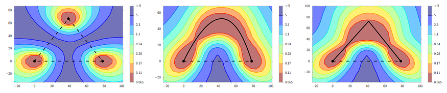
The next step came in an earlier paper from Vetrov’s lab. In “Loss Surfaces, Mode Connectivity, and Fast Ensembling of DNNs”, Garipov et al. showed that for a wide range of architectures, their local optima are actually connected by rather simple curves along which the loss remains near-constant! Here is an illustration:
Garipov et al. show that if you train three different networks you’ll get a landscape like the one shown on the left, as you would expect. But if you then use their proposed mode connecting procedure, you can find curves of near-constant loss function that connect the dots. On the plots, the X-axis is always the same but Y-axes are different, and the procedure invariably finds a valley that connects the two optima.
Based on this observation, Garipov et al. proposed a new ensembling procedure, Fast Geometric Ensembling (FGE), which basically amounts to averaging the weights along such a mode connecting path.
Still, this was rather computationally intensive: you had to find several local optima, then connect them with a separate computational procedure. And, ultimately, it’s still an ensemble: you need to keep multiple models, run them all at inference time, and then average their answers. Stochastic Weight Averaging (SWA), proposed by Izmailov et al. in the paper in question, does away with most of these extra costs!
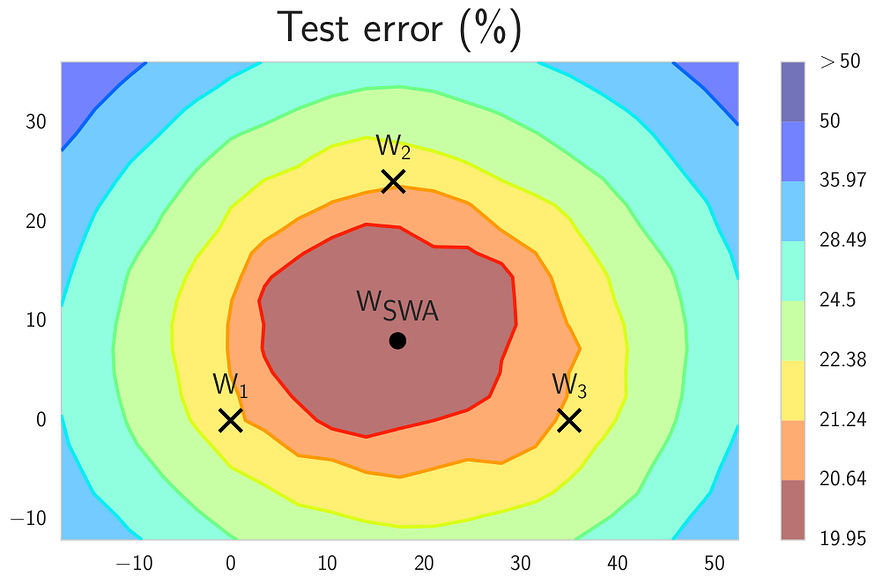
This time, the fundamental observation is that stochastic gradient descent with cyclical and constant learning rates actually traverses the regions in the weight space corresponding to high-performing networks, but it does not reach the central points of these regions. That is, three networks averaged out by FGE would most likely look something like this:
So instead of averaging their predictions, why not average the weights directly, getting to the wonderful wSWA point shown above?! That’s exactly what stochastic weight averaging does:
start with a (somewhat) pretrained model;
keep training with a cyclical or constant learning rate schedule;
on every iteration of training, add the current vector to a separately accumulating running average.
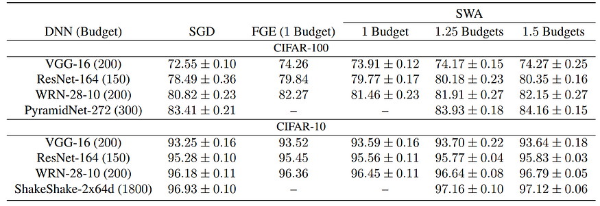
And that’s it! The results are nothing short of amazing: with no additional cost at inference time and very little cost at training time, SWA actually manages to improve virtually all architectures across a wide variety of datasets and settings. Here is a sample of experimental results:
SWA is a straightforward drop-in replacement for stochastic gradient descent, and, naturally, it has an official github repository released by the authors. Try it out and share your results in the comments!
Conclusion
This has been a rather challenging NeuroNugget, I’m afraid, and we have only skimmed the surface of several latest papers by Dmitry Vetrov and his group.
I have tried to outline the main ideas that each paper brings to deep learning, but the most important thing I want to emphasize is the common thread: each paper we have considered today presents a novel idea that looks plausible, works well (at least on toy examples, sometimes more experiments are needed before it can be used in large-scale networks), and opens up a whole new direction of study, usually somewhere near the field of Bayesian deep learning.
That’s how Dmitry Vetrov has always done research: he has a vision and a knack for finding these “paths less traveled” in the forest of deep learning, a forest that by now might seem rather well-trodden. Still, he did it in 2009, he is doing it in 2019, and I’m sure he will still be finding completely novel ideas and uncovering new directions in 2049. Thank you Dmitry — and good luck!
Sergey Nikolenko Chief Research Officer, Neuromation
Last time, we had some very serious stuff to discuss. Let’s touch upon a much lighter topic today: anime! It turns out that many architectures we’ve discussed on this very blog, or plan to discuss in more detail in the future, have already been applied to Japanese-style comics and animation.
Let me start by giving a shout out to the owner of this fantastic github repository. It is the most comprehensive resource for all things anime in deep learning. Thanks for putting this together and maintaining it, whoever you are!
We will be mostly talking about generating anime characters, but the last part will be a brief overview of some other anime-related problems.
Do everything by hand, even when using the computer.
Hayao Miyazaki
Drawing Anime Characters with GANs
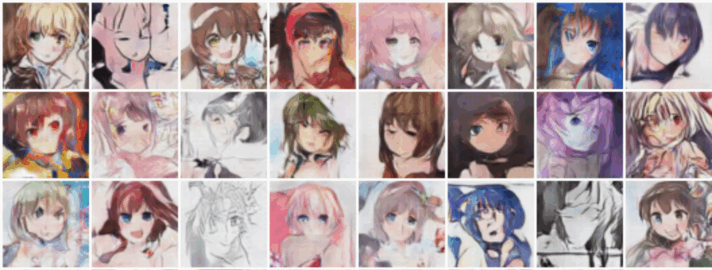
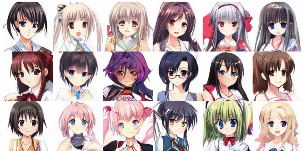
Guess who drew the characters you saw above? You guessed right, there was no manga artist who thought them up, they were drawn automatically with a generative model.
The paper by Jin et al. (2017) presents an architecture based on generative adversarial models trained to generate anime characters. We have spoken about GANs several times on this blog (see, e.g., here or here), and this sounds like a relatively straightforward application. But attempts at direct applications of basic GAN architectures such as DCGAN for this problem, even a relatively successful attempt called (unsurprisingly) AnimeGAN, produced only low-resolution, blurry and generally unsatisfactory images, e.g.:
How did Jin et al. bridge the gap between this and what we saw above?
First, let’s talk about the data. This work shows a good example of a general trend: dataset collection and especially labeling increasingly becomes an automated or at least semi-automated process, using models that we believe to work reliably in order to label datasets for more complex models.
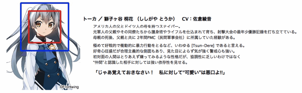
To get a big collection of anime character faces, Jin et al. scraped the Getchu website that showcases thousands of Japanese games, including unified presentations of their characters, in good quality and on neutral background:
On these pictures, they ran a face detection model called lbpcascade, specifically trained to do face detection for anime/manga, and then enlarged the resulting bounding box (shown in red above) by 1.5x to add some context (shown in blue above). To add the “semi-” to “semi-automated”, the authors also checked the resulting 42000 images by hand and removed about 4% of false positives They don’t show a comparison but I’m sure this was an important step for data preparation.
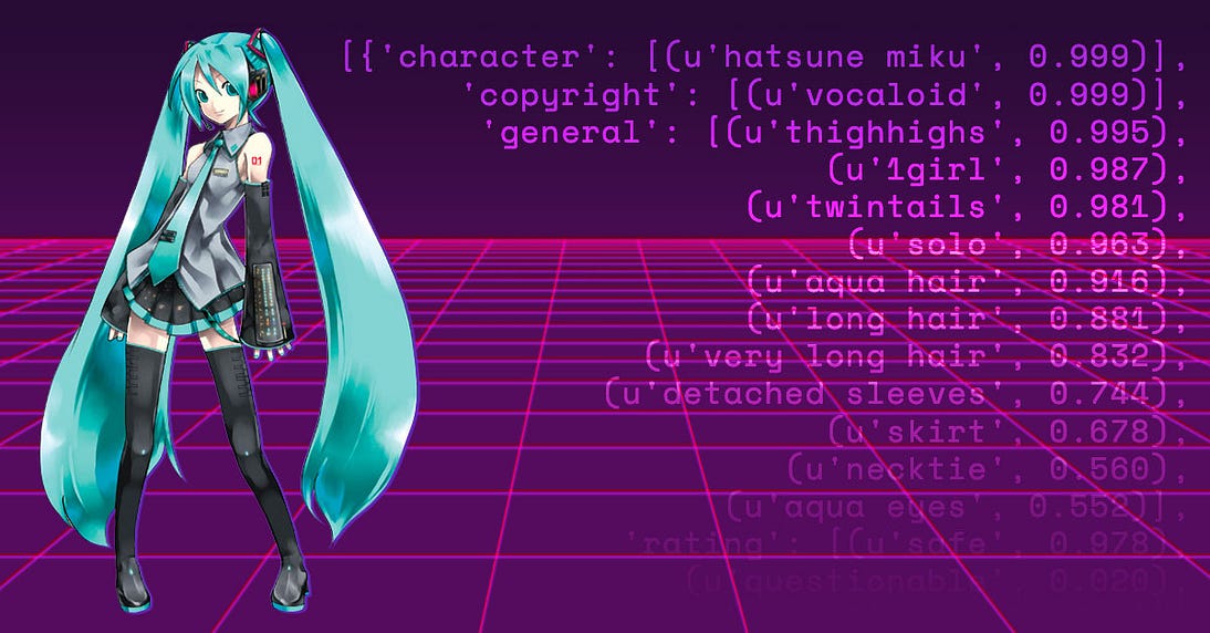
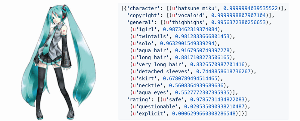
But that’s not all. Jin et al. wanted to have conditional generation, where you would be able to get a blonde anime girl with a ponytail or a brown-eyed red-haired one with glasses. To do that, they ran a pretrained model called Illustration2Vec which is designed to predict a large number of predefined tags from an anime/manga image. Here is a sample:
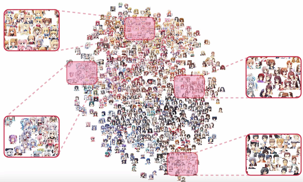
Jin et al. chose suitable thresholds for the classifiers in Illustration2Vec, but basically they used this pretrained model as is, relying on its accuracy to create the training set for the GAN. This is an interesting illustration to how you can bootstrap training sets from pretrained models: it won’t always work but when it does, it can produce large training sets very efficiently. As a result, they now had a large dataset of images labeled with various tags, with a feature vector associated with every image. Here is a part of this dataset in tSNE visualization of the feature vectors:
The next step would be to choose the GAN architecture. Jin et al. went with DRAGAN (Deep Regret Analytic Generative Adversarial Networks), an additional loss function suggested by Kodali et al. (2017) to alleviate the mode collapse problem. We will not go into further details on DRAGAN here. Suffice it to say that the final architecture is basically a standard GAN with a generator and a discriminator, and with some additional loss functions to account for the DRAGAN gradient penalty and for the correct assignment of class labels to make it conditional. The architectures for both generator and discriminator are based on SRResNet, pretty standard convolutional architectures with residual connections.
So now we have both the data and the architecture. Then we train for a while, and then we generate!
Those were the results of unconditional generation, but we can also set up some attributes as conditions. Below, on the left we have the “aqua hair, long hair, drill hair, open mouth, glasses, aqua eyes” tags and on the right we have “orange hair, ponytail, hat, glasses, red eyes, orange eyes”:
And, even better, you can play with this generative model yourself. Jin et al. made the models available through a public frontend at this website; you can specify certain characteristic features and generate new anime characters automatically. Try it!
Next Step: Full-Body Generation with Pose Conditions
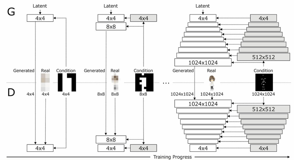
Hamada et al. (2018) take the next step in generating anime characters with GANs: instead of just doing a head shot like Jin et al. above, they generate a full-body image with a predefined pose. They are using the basic idea of progressively growing GANs from Karras et al. (2018), a paper that we have actually already discussed in detail on this very blog:
begin with training a GAN to generate extremely small images, like 4×4 pixels;
use the result as a condition to train a GAN that scales it up to 8×8 pixels, a process similar to superresolution;
use the result as a condition to train a GAN that scales it up to 16×16 pixels…
…and so on until you get to 1024×1024 or something like that.
The novel idea by Hamada et al. is that you can also use the pose as a condition, first expressing it in the form of a pixel mask and then scaling it down to 4×4 pixels, then 8×8, and so on:
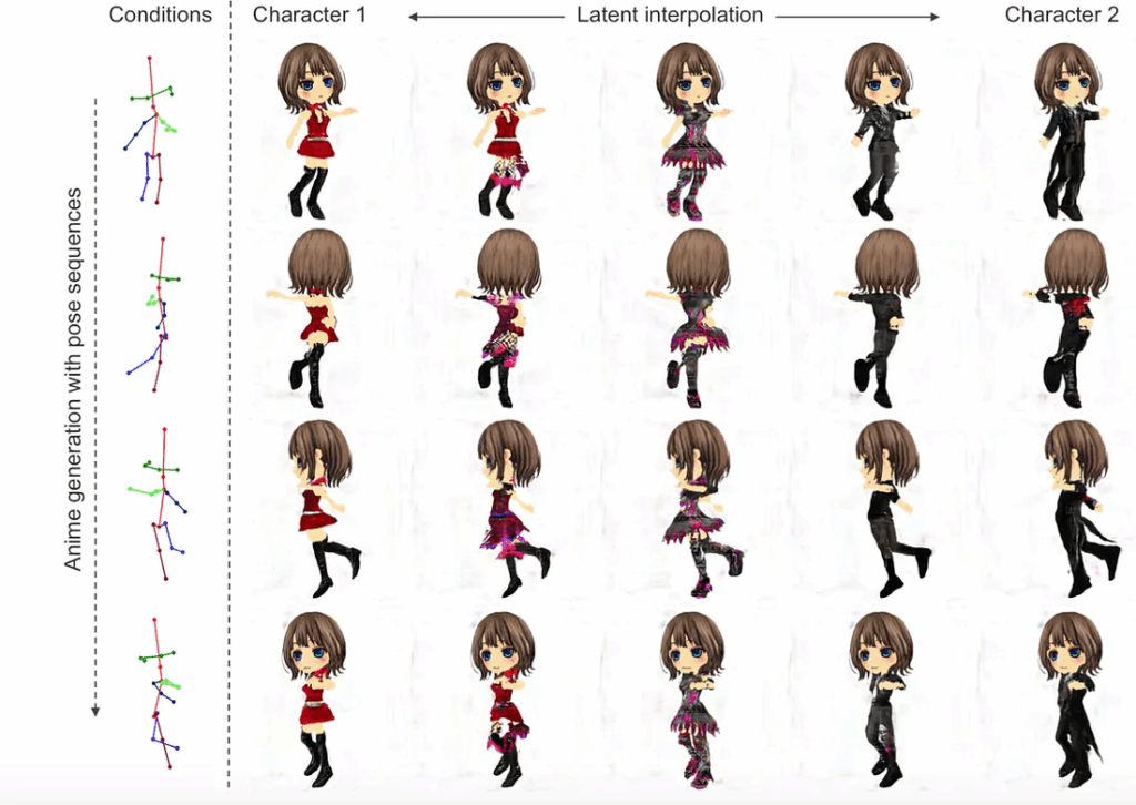
And as a result, the progressive structure-conditional GAN is able to generate nice pictures with predefined poses. As usual with GANs you can interpolate between characters while keeping the pose fixed, and you can produce different poses of the same character, which makes this paper a big step towards developing a tool that would actually help artists and animators. Here is a sample output:
Have you seen thispersondoesnotexist.com? It shows fake people generated by the latest and greatest GAN-based architecture for face generation, the StyleGAN, and it’s been all over the Web for a while.
Well, turns out there is an anime equivalent! thiswaifudoesnotexist.net generates random anime characters with the StyleGAN architecture and even adds a randomly generated plot summary! Like this:
Looks even better! But wait, what is this StyleGAN we speak of?
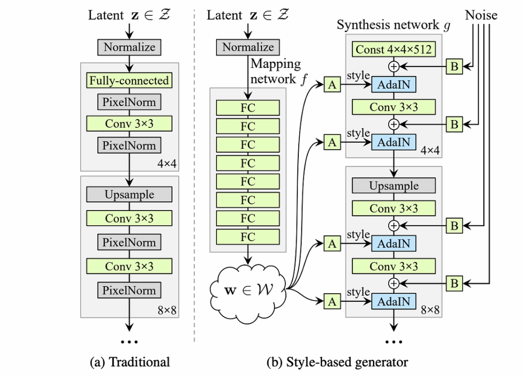
StyleGAN is an architecture by NVIDIA researchers Karras et al. (2018), the same group who had previously made progressively growing GANs. This time, they kept the stack of progressive superresolution but changed the architecture of the basic convolutional model, making the generator similar to style transfer networks. Essentially, instead of simply putting a latent code through a convolutional network, like traditional GANs do, StyleGAN first recovers an intermediate code vector and then uses it several times to inform the synthesis network, with external noise coming in at every level. Here is a picture from the paper, with a traditional generator architecture on the left and StyleGAN on the right:
We won’t go into more detail on this here, as the StyleGAN would deserve a dedicated NeuroNugget to explain fully (and maybe it’ll get it). Safe to say that the final result now looks even better. StyleGAN defines a new gold standard for face generation, as shown on thispersondoesnotexist.com and now, as we can see, on thiswaifudoesnotexist.net. As for the text generation part, this is a completely different can of worms, awaiting its own NeuroNuggets, quite possibly in the near future…
Brief Overviews
Let us close with a few more papers that solve interesting anime/manga-related problems.
Style transfer for anime sketches. We’ve spoken of GANs that use ideas similar to style transfer, but what about style transfer itself? Zhang et al. (2017) present a style transfer network based on U-Net and auxiliary classifier GAN (AC-GAN) that can fill in sketches with color schemes derived from separate (and completely different) style images. This solves a very practical problem for anime artists: if you can draw a character in full color once and then just apply the style to sketches, it would be a huge saving of effort. We are not quite there yet, but look at the results; in the three examples below, the sketch shown in the top left is combined with a style image shown in the bottom left to get the final image:
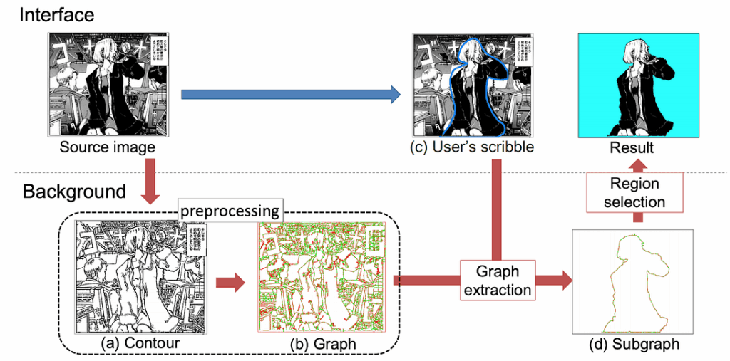
Interactive segmentation. Ito et al. (2016) propose an interactive segmentation method intended for manga. An important problem for manga illustrators would be to have automated or semi-automated segmentation tools, so they can cut out individual characters or parts of the scene from existing drawings. That’s exactly what Ito et al. do (without any deep learning, by the way, by improving classical segmentation techniques):
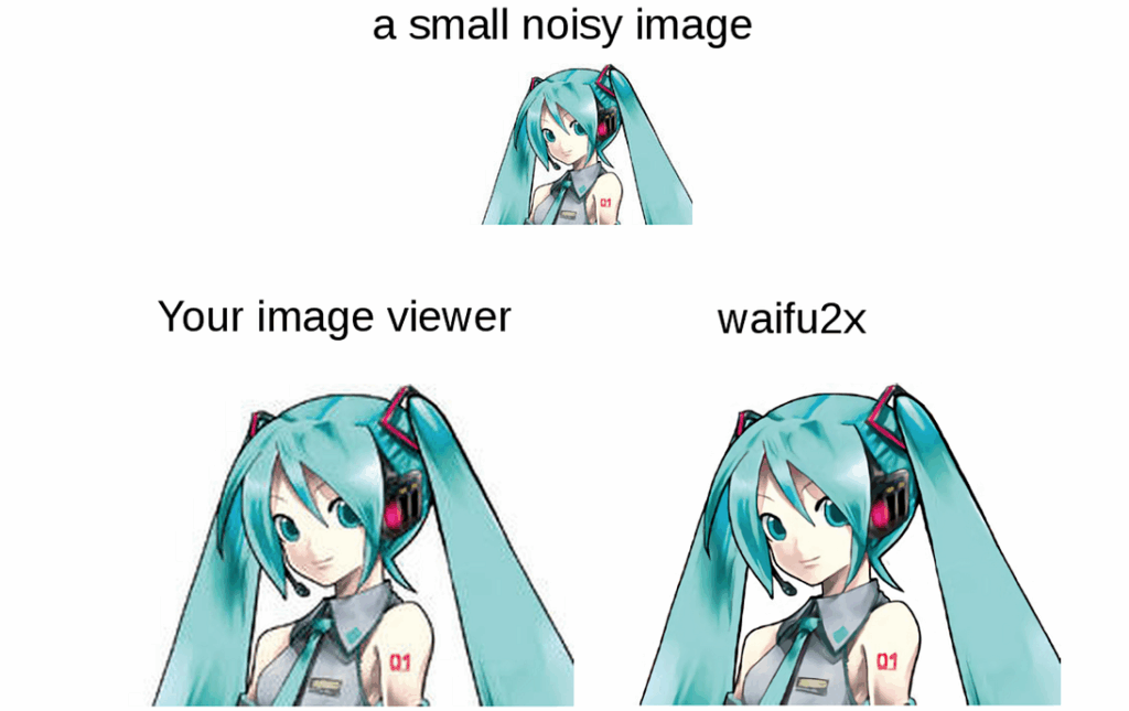
Anime superresolution. We have already mentioned superresolution as a stepping stone in progressively growing GANs, but one can also use it directly to transform small and/or low-res images to high-quality anime. The waifu2x model is a model based on SRCNN (single-image superresolution based on convolutional neural networks) that is a little bit fine-tuned and extensively pre-trained to handle anime. The results are actually pretty impressive — here is how waifu2x works:
Cartoons in general and anime in particular represent a very nice domain for computer vision:
images in anime style are much simpler than real-life photos: the edges are pronounced, the contours are mostly perfectly closed, many shapes have a distinct style that makes them easy to recognize, and so on;
there is a natural demand for the tools to manipulate anime images from anime artists, animators, and enthusiasts;
as we have seen even in this post, there exist large databases of categorized and tagged images that can be scraped for datasets.
So no wonder people have been able to make a lot of things work well in the domain of anime. Actually, I would expect that anime might become an important frontier for image manipulation models, a sandbox where the models work well and do cool things before they can “graduate” to realistic photographic imagery.
But to do that, the world needs large-scale open datasets and a clear formulation of the main problems in the field. Hopefully, the anime community can help with that, and then I have no doubt researchers all over the world will jump in… not only because it might be easier than real photos, but also simply because it’s so cool. Have fun!
Sergey Nikolenko Chief Research Officer, Neuromation
New Year celebrations are just behind us, but things are already happening in 2019. One very exciting development for machine learning researchers all around the world is the new journal from the venerable Nature family: Nature Machine Intelligence. Its volume 1 is dated January 2019, and it’s already out (all papers are in open access, you can read them right there). Machine learning results have already made it into Nature — for example, I’ve always wondered how a paper about a piece of software playing a boardgame is about Nature. But now we have a new top venue specifically devoted to machine learning.
Nature Machine Intelligence begins on a high note. We might go back to its first volume in later installments, but today I want to discuss one especially unexpected and exciting result: a paper by Ben-David et al. called Learnability Can Be Undecidable. It brings into our humble and so far very practical field of science: Godel’s incompleteness theorem.
Independence Results: Things We Cannot Know
They might or they might not. You never can tell with bees.
A.A. Milne
Mathematical logic is a new subject for our series, and indeed it doesn’t appear too often in the context of machine learning. So let’s start with a brief introduction.
Gödel’s incompleteness theorem establishes that in any (sufficiently complex) formal system, there are things we can neither prove nor disprove. A formal system is basically a set of symbols and axioms that define relations between these symbols. For example, you can have two functions, + and *, and constants 0 and 1, with the usual axioms for addition and multiplication that define a field. Then you can have models of this formal system, i.e., interpretations of the symbols such that all axioms hold. As an example, the set of real numbers with standard interpretations of 0,1,+,* is one model of the theory of fields, and the set of rational numbers is another.
The original constructions given by Gödel are relatively involved and not easy to grasp without a logical background. They have been quite beautifully explained for the layperson in Douglas Hofstadter’s famous book Gödel, Escher, Bach, but it does take a few dozen pages, so we won’t go into that here.
How can you prove that a certain statement is unprovable? Sounds like an oxymoron, but the basic idea of many such proofs is straightforward: you construct two models of the formal system such that in one of them the statement is true and in the other it’s not.
For example, consider a very simple formal system with only one function s(x), which we interpret as “taking the next element”, and one constant 0. We can construct formulas (terms, to be precise) like s(0), s(s(0)), s(s(0)) etc. We can think of them as natural numbers: 1:=s(0), 2:=s(1)=s(s(0)), and so on. But do negative numbers also exist? Formally, is there an x such that s(x)=0?
The question makes sense (it’s easy to write as a logical formula: ∃x s(x)=0) but has no answer. First, the set of natural numbers 0,1,2,… is a valid model for this formal system, with the function s defined as s(x)=x+1. And in this model, the answer is no: there is no number preceding zero. But the set of integers …,-2,-1,0,1,2,… is also a valid model, with the same interpretation s(x)=x+1! And now, we clearly have s(-1)=0. This means that the original formal system does not know whether negative numbers exist.
Of course, this was a very, very simple formal system and nobody really expected it to have answers to complicated questions. But the same kind of reasoning can be applied to much more complex systems. For example, the axioms of a field in mathematics do not have an answer to whether irrational numbers exist; e.g., ∃x(x*x=2) is true in the real numbers but false in the rational numbers, and both are fields. Godel’s incompleteness theorem says that we can find such statements for any reasonably powerful formal system, including for example, Zermelo-Fraenkel set theory (ZFC), which is basically what we usually mean by mathematics. Logicians have constructed statements that are independent of ZFC axioms.
One such statement is the famous continuum hypothesis. Modern mathematical logic was in many ways initiated by Georg Cantor, who was the first to try to systematically develop the foundations of mathematics, specifically formal and consistent set theory. Cantor was the first to understand that there are different kinds of infinities: the set of natural numbers is smaller than the set of reals because you cannot enumerate all real numbers. The cardinality (size) of the set of natural numbers, denoted ℵ₀ (“aleph-null”) is the smallest infinite number (smallest infinite cardinal, as they are called in mathematical logic), and the set of reals is said to have the cardinality of continuum, ℵ₁ (“aleph-one”).
There is no doubt that ℵ₁ > ℵ₀, but is there anything in between the natural numbers and the reals? This is known as the continuum hypothesis: it says that ℵ₁ is the smallest infinite cardinal larger than ℵ₀. And it turns out to be independent of ZFC: you can construct a model of mathematics where there is an intermediate cardinality, and you can construct a model where there isn’t. There is really no point to ask which model we live in: it’s unclear if there is anything truly infinite in our world at all.
Undecidability in Machine Learning
Some problems are so complex that you have to be highly intelligent and well informed just to be undecided about them.
Laurence J. Peter
Okay, so what does all of this have to do with machine learning? In our field, we usually talk about finite datasets that define optimization problems for the weights. How can we find obscure statements about the existence of various infinities within our practical and usually well-defined field?
Ben-David et al. speak about the “estimating the maximum” problem (EMX):
Given a family F of subsets of some domain X, find a set F whose measure with respect to an unknown probability distribution P is close to maximal, based on a finite sample generated independently from P.
Sounds complicated, but it’s really just a general formulation of many machine learning problems. Ben-David et al. give the following example: suppose you are placing ads on a website. The domain X is the set of visitors for the website, every ad A has its target audience Fᴬ, and P is the distribution of visitors for the site. Then the problem of finding the best ad to show is exactly the problem of finding a set Fᴬ that has the largest measure with respect to P, i.e., it will most probably resonate with a random visitor.
In fact, EMX is a very general problem, and its relation to machine learning is much deeper than this example shows. You can think of a set F as a function from the domain X to 0 and 1: F(x)=1 if x belongs to F and F(x)=0 if it doesn’t. And the EMX problem is asking to find a function F from a given family that tries to maximize the expectation Eᴾ(F) with respect to the distribution P.
Let us now think of samples from the distribution P as data samples, and treat the functions as classifiers. Now the setting begins to make a lot of sense for machine learning: it means that you can know the labels of all data samples and need to, given a sample of the data, find a classifier from a given family that will have low error with respect to the data distribution. Sounds very much like a standard machine learning problem, right? For more details on this setting, check out an earlier paper by Ben-David (two Ben-Davids, actually).
Ben-David et al. consider a rather simple special case of the EMX problem, where X is the interval [0,1] and the family of subsets are all finite subsets of X, that is, finite collections of real numbers from [0,1]. They prove that the problem of EMX learnability with probability 2/3, that is, given some i.i.d. samples from a distribution P, find a finite subset of [0,1] that has probability at least 2/3, is independent of ZFC! That is, our regular mathematics cannot say whether you can find a good classifier in this setting. They do it by constructing a (rather intricate) reduction of the continuum hypothesis to this case of EMX learnability.
So What’s the Takeaway?
A conclusion is the place where you got tired thinking.
Martin H. Fischer
The results of Ben-David et al. are really beautiful. They connect a lot of dots: unprovability and independence, machine learning, compression schemes (used in the proof), and computational learning theory. One important corollary the paper’s main result is that there can be no general notion of dimension for EMX learnability, like the VC (Vapnik-Chervonenkis) dimension is for PAC learnability. I have no doubt these ideas will blossom into a whole new direction of research.
Still, as it sadly often happens with mathematical logic, this result can leave you a bit underwhelmed. It only makes sense in the context of uncountable sets, which you can hardly find in real life. Ben-David et al. themselves admit in the conclusion that the proof hinges on the fact that EMX asks to find a function over an infinite domain rather than, say, an algorithm, which would be a much simpler object (in theoretical computer science, algorithms are defined as Turing machines, basically finite sets of instructions for a very simple formalized “computer”, and there are only countably many finite sets of instructions while there are, obviously, a continuum of finite subsets of [0,1] and hence functions).
Nevertheless, it is really exciting to see different fields of mathematics connected in such unexpected and beautiful ways. I hope that more results like this will follow, and I hope that in the future, modern mathematics will play a more important role in machine learning than it does now. Thank you for reading!
Sergey Nikolenko Chief Research Officer, Neuromation
It’s been quite a while, but the time has finally come to return to the story of deep learning for drug discovery, a story we began in April. Back then, I presented to you the first paper that had an official Neuromation affiliation, “3D Molecular Representations Based on the Wave Transform for Convolutional Neural Networks”, published in a top biomedical journal Molecular Pharmaceutics. By now, researchers from Neuromation have published more than ten papers, we have told you about some of them in our Neuromation Research blog posts, and, most importantly, we have already released our next big project in collaboration with Insilico, the MOSES dataset and benchmarking suite. But today, we finally come back to that first paper. Once again, many thanks to the CEO of Insilico Medicine Alex Zhavoronkov and CEO of Insilico Taiwan Artur Kadurin who have been the main researchers on this topic. I am very grateful for the opportunity to work alongside them in this project.
A Quick Recap: GANs for Drug Discovery
For a more detailed introduction to the topic, you are welcome to go back and re-read the first part; but to keep this one self-consistent, let me begin with a quick reminder.
Drug discovery is organized like a highly selective funnel: at the first stage, you have doctors coming up with the properties that a molecule should have to be a good drug (binding with a given protein, dissolving in water and so on) and then with plausible candidates for molecules that might have these properties. Then these lead molecules are sent to the lab, and if they survive pre-clinical studies, they go to the official process of clinical trials and, finally, approval of the FDA or similar bodies in other countries.
Only a tiny part of the lead molecules will ever get FDA approval, and the whole process is extremely expensive (developing a new drug takes about 10 years and costs $2.6 billion on average), so one of the main problems of modern medicine is to try and make the funnel as efficient as possible on every stage. Deep learning for drug discovery aims to improve the very first part, generating lead molecules. We try to develop generative models that will produce plausible candidates with useful properties.
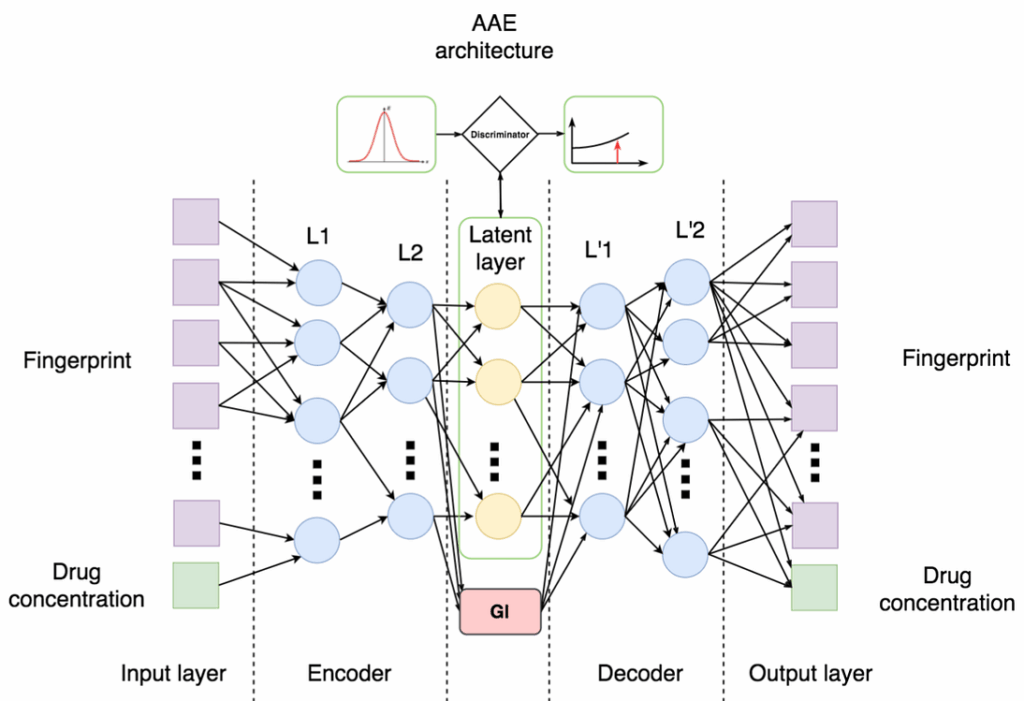
This is, in essence, a so-called conditional adversarial autoencoder:
an autoencoder receives as input a SMILES fingerprint (basically a bit string that represents a molecule and makes a lot of chemical and biological sense) and the drug concentration; it learns to produce a latent representation (embedding) on the middle layer and then decode it back to obtain the original fingerprint;
the condition (GI on the bottom) encodes the properties of the molecule; the conditional autoencoder trains on molecules with known properties, and then can potentially generate molecules with desired combinations of properties by supplying them to the middle layer;
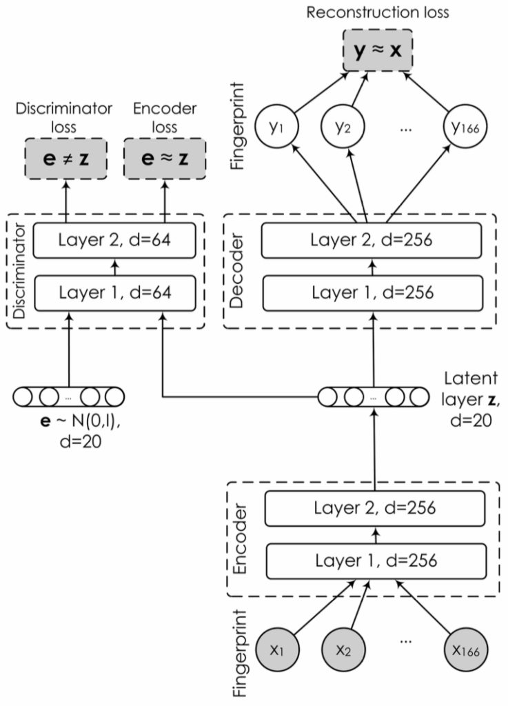
and, finally, the discriminator (on top) tries to tell apart the distribution of latent representations (embeddings) and some known distribution, e.g., a standard Gaussian; this is the main idea of AAE that is supposed to make an autoencoder into a generative model: if we can make the distribution of embeddings indistinguishable from a known distribution, we can sample from the known distribution and decode these samples to get reasonable objects.
Again, we have been through this in the first part, so I refer there for more details. But today, we go further.
druGAN: AAE or VAE?
Our next paper on generative models for drug discovery had a laconic title of “druGAN: An Advanced Generative Adversarial Autoencoder Model for de Novo Generation of New Molecules with Desired Molecular Properties in Silico”, and it appeared in Molecular Pharmaceutics in 2017. The Cornucopia paper that we reviewed above actually solved a relatively small and limited problem: the conditional AAE was trained on a dataset with only 6252 available compounds profiled on a single cell line (MCF-7). This limited scope, naturally, could not satisfy the ambitious team of Insilico Medicine. And it only considered one type of generative models, GANs… wait, what? There’s more?
Well yes, there is! There exists a wide variety of generative models even if you concentrate only on deep learning, i.e., models that have neural networks somewhere. I recommend the well-known tutorial by Ian Goodfellow: a lot has happened in GANs since that tutorial but the taxonomy of generative models is still very relevant.
One of the main classes of generative models in deep learning today are variational autoencoders (VAE). The idea of VAE is exactly the same as in AAE: we want to make the distribution of latent embeddings z similar to some known distribution (say, a Gaussian) so that we can sample embeddings directly and then decode to get sample objects. But VAE implements this idea in a completely different way.
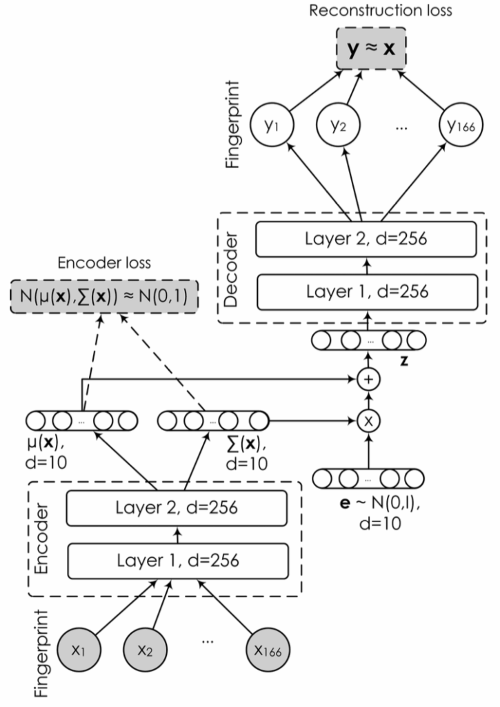
VAE makes the assumption that the embeddings are indeed normally distributed, z ~ N(μ, Σ), where μ is the mean and Σ is the covariance matrix. The job of the encoder now is to produce the parameters of this normal distribution given an object, that is, the encoder outputs μ(x) and Σ(x) for the input object x; Σ is usually assumed to be diagonal, so it’s basically a vector of dimension 2d, where d is the dimension of z. VAE also adds a standard normal prior distribution on μ(x) and Σ(x). Then VAE samples a vector z from the distribution N(μ(x), Σ(x)), decodes it back to the original space of objects and, as a good autoencoder should, tries to make the reconstruction accurate. Here is how it all comes together in the druGAN paper:
Notice how z is not sampled directly from N(μ(x), Σ(x)) but rather comes from a standard normal distribution which is then linearly transformed by μ(x) and Σ(x). This is known as the reparametrization trick, and it was one of the key ideas that made VAEs possible.
I’m not being entirely honest here: there is some beautiful mathematics behind all this, and it is needed to make this work, but, unfortunately, it goes way outside of the format of a popular article. Still, I recommend explanations such as this one, and maybe one day we will have a detailed NeuroNugget about it.
In the druGAN paper, Kadurin et al. compared this VAE with an AAE-based architecture, an improved modification of the one proposed in the Cornucopia paper. Here is the architecture; comparing it with the picture above, you can see the difference between AAE and VAE:
We trained several versions of both VAE and AAE on a set of MACCS fingerprints produced from the PubChem database of substances that contains more than 72 million different molecules, quite a step up from the six thousand used in Cornucopia. The results were promising: we were able to sample quite varied molecules and also trained a simple linear regression that predicted solubility from the features extracted by the autoencoders. Generally, the best AAE models outperformed the best VAE models, although the latter had some advantages in certain settings.
The most meaningful conclusion, however, was that we always had a tradeoff between two most important metrics: quality of reconstruction (measured by the reconstruction error) and variability of the molecules sampled from the trained model (measured by various diversity metrics). Without the former, you don’t get good molecules; without the latter, you don’t get new molecules. This tradeoff lies in the heart of modern research on generative models, and it is still very hard to keep the results both reasonable and diverse.
Molecules in 3D: the Wave Transform Representation
This work had a slightly different emphasis: instead of devising and testing new architectures, we tried to look at the descriptions of molecules that are fed as input to these architectures. One motivation for this was that the entire framework of deep learning for drug discovery that we had seen in both Cornucopia and druGAN presupposes that we will screen predicted fingerprints against a database of existing molecules. Not all fingerprints are viable, so you cannot take an arbitrary MACCS fingerprint and reconstruct a real molecule: you have to screen against actually existing fingerprints and find the best matches among them. If we could use a more informative molecular representation, we might not have to choose the proposed molecules from a known database, leading to the holy grail of drug discovery: de novo generation of molecular structures.
So how can we encode molecular structure? People have tried a lot of things: a comprehensive reference by Todeschini et al. (2009) lists several thousand of molecular descriptors, and this list has grown even further over the last decade. They can be broken down into string encodings, such as MACCS itself, graph encodings that capture the molecular graph (there are some very interesting works on how to make convolutions on graphs, e.g., (Kearns et al., 2016; Liu et al., 2018)), and 3D representations that also capture the bond lengths and mutual orientation of atoms in space.
In molecular biology and chemistry, the 3D structure of a molecule is called a conformation; a given molecule can have many different conformations, and it may turn out that it’s important to choose the right one. For example, is the part of the molecule that is supposed to bind with a protein gets hidden inside the rest of the molecule, and the drug will simply not work. So it sounds like a good idea to feed our models with 3D structures of the molecules in question: after all, it’s basically a picture in 3D, and there are plenty of successful CNNs with 3D input.
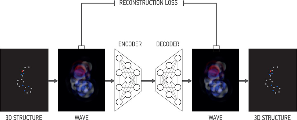
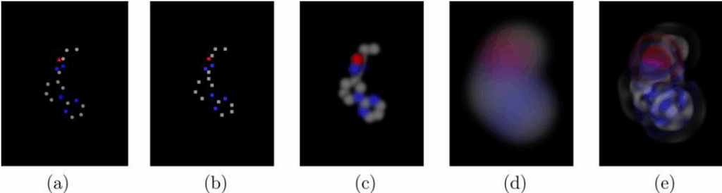
But it proves to be not that easy. Let’s look at the main picture from the paper:
Part (a) shows how the original molecule looks in 3D space: it’s a 3D structure composed of different atoms shown in different colors on the picture. How do we represent this structure to feed it to convolutional networks? The most straightforward answer would be to discretize the space into voxels (fun fact: the linear size of a voxel here is 0.5Å; that’s Angstrem, 0.1 nanometers!) and represent each atom as a one-hot representation in the voxel; the result is shown in part (b).
But this representation is far from perfect. First, it’s very sparse: less than 0.1% of the voxels contain atoms. Second, due to this sparsity interactions between atoms are also hard to capture: yes, some atoms are near each other and some are farther away, but there is a lot of empty space around atoms, the data does not have enough redundancy, and CNNs just don’t work too well with this kind of data. Sparse voxels lead to sparse gradients, and the whole thing underfits.
In the paper, we proposed a different kind of “blurring” based on the wave transform; its kernel is a Gaussian multiplied by a cosine function of the distance to center, so the “ball” still decays exponentially but now spreads out in waves. The result is shown in part (e) above. In the paper, we show that this transform has better theoretical properties, deriving an analytical inverse operation (deconvolution) for the wave transform.
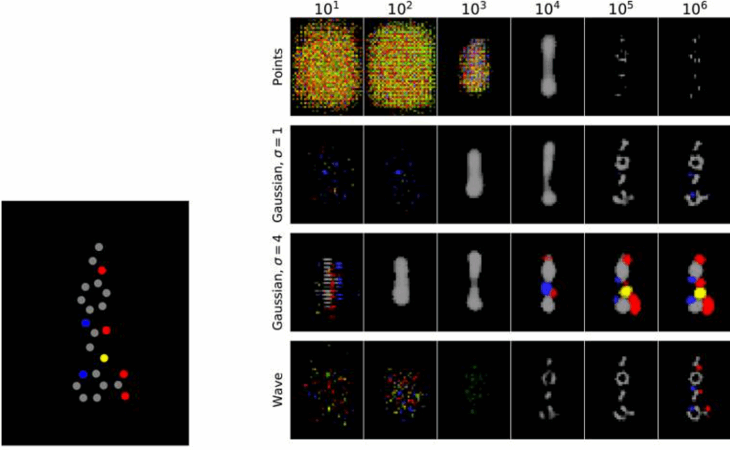
This converts to practical advantages, too. In the paper, we trained a simple autoencoder based on the Xception network, but even with this experiment you can see how the wave transform representation performs better. The picture below shows reconstruction results from the autoencoder at different stages of training:
We can see that the voxel-based representation never allowed to reconstruct anything except carbon (and even that quite poorly), and Gaussian blur added nitrogen; the wave transform, however, has also been able to reconstruct oxygen atoms, and the general structure looks much better as well. Our experiments have also shown that the wave transform representation outperforms others in classification problems, e.g., in reconstructing the bits from MACCS fingerprints.
Conclusion
In this post, we have seen how different generative models compare for generating molecules that might become plausible candidates for new drugs. Insilico Medicine is already testing some of these molecules in the lab. Unfortunately, it’s a lengthy process, and nothing is guaranteed; but I hope we will soon see some of the automatically generated lead molecules confirmed by real experiments, and this may completely change medicine as we know it. Best of luck to our friends and collaborators from Insilico Medicine, and I’m sure we will meet them again in future NeuroNuggets. Stay tuned!
Sergey Nikolenko Chief Research Officer, Neuromation
Our long-term collaboration with Insilico Medicine, a company that focuses on artificial intelligence for drug discovery and longevity research, has borne some very important fruit. We have released a benchmarking platform for generative models, which we named MOSES (MOlecular SEtS). You can find the paper currently released on arXiv, the github repository, and the press release by research partner Insilico. Congratulations to the whole team! Before we dive into a little bit of detail, here is the Neuromation staff together with our collaborators from Insilico at the NIPS (NeurIPS, as they call it now) conference currently held in Montreal:
Neuromation and Insilico Medicine at NIPS 2018. Left to right: Alex Zhavoronkov (Insilico/Buck Institute for Research on Aging), Elena Tutubalina (Neuromation), Daniil Polykovsky, Polina Mamoshina (Insilico), Rauf Kurbanov (Neuromation).
So what is MOSES, why do we care, and what do Neuromation and Insilico have in common here?
MOSES is a benchmarking platform for generative models that aim to generate molecular structures. We covered generative models such as generative adversarial networks (GANs) before (e.g., here or here). In molecular biology and biochemistry, generative models are used to produce candidate compounds that might have desired qualities. We have already published a post about our previous joint project with Insilico which provides more details about such models.
One common thread in generative models is that they are really difficult to evaluate and compare. You have a black box that produces, say, images of human faces. Scratch that, you have twenty black boxes. Which one is best? You could try to get closer to the true answer by asking real people to evaluate the faces, but this surely won’t scale.
So researchers have been developing metrics to compare generative models. I will save a more detailed explanation of the metrics for an in-depth Neuromation Research post which is going to follow soon. For now, let me just say that there are plenty of different metrics. It’s really hard to collect them all from very different implementations, and even harder to claim that your numbers are really comparable with the numbers in other papers. The whole field could sure use some standardization and streamlining.
That’s where MOSES comes in. In this project, we:
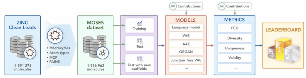
prepared a large dataset of approximately 2 million molecules based on specially designed chemical filters;
implemented the most popular metrics for the evaluation of generative models;
most importantly, implemented several state of the art models and provided a large and unified experimental comparison between them.
The MOSES pipeline
Building MOSES was a big project. We have been working on it for the better part of this year; 40 weeks in the title are no exaggeration. In a project like that, you need a deep and well integrated collaboration between chemists, medical researchers, and machine learning gurus. And that is exactly what we had between Neuromation, Insilico Medicine, the Harvard University and the University of Toronto.
The result is a benchmarking dataset, an evaluation pipeline, and a large-scale experimental comparison that provides the stable footing so badly needed for this field. Now, new works can build upon this foundation, compare new models with baselines from our paper, and make direct quantitative comparisons in terms of various evaluation metrics. We hope that researchers all over the world will benefit from our joint effort.
My congratulations to our team and to our dear friends at Insilico Medicine! Lots of contributors, but let me please highlight and thank the following individuals: big thanks to Daniil Polykovsky, Alexander Zhebrak, Vladimir Aladinskiy, Mark Veselov, Artur Kadurin, and Alex Zhavoronkov from Insilico, to Benjamin Sanchez-Lengeling from Harvard, Alan Aspuru-Gusik from the University of Toronto/Vector Institute, and to Neuromation researchers Sergey Golovanov, Oktai Tatanov, Stanislav Belyaev, Rauf Kurbanov, and Aleksey Artamonov. Thanks guys!
Thank you for reading and stay tuned for the next updates from our Neuromation Research blog!
Sergey Nikolenko Chief Research Officer, Neuromation
…Many people think that authors just cut and paste from real life into books. It doesn’t work quite that way. ― Paul Fleischman
As the CVPR in Review posts (there were five: GANs for computer vision, pose estimation and tracking for humans, synthetic data, domain adaptation, and face synthesis) have finally dried up, we again turn to our usual stuff. In the NeuroNugget series, we usually talk about specific ideas in deep learning and try to bring you up to speed on each. We have had some pretty general and all-encompassing posts here, but it is often both fun and instructive to dive deeper into something very specific. So we will devote some NeuroNuggets to reviewing a few recent papers that share a common thread.
And today, this thread is… cut-and-paste! And not the kind we all do from other people’s GitHub repositories. In computer vision, this idea is often directly related to synthetic data, as cutting and pasting sometimes proves to be a fertile middle ground between real data and going fully synthetic. But let’s not get ahead of ourselves…
Naive Cut-and-Paste as Data Augmentation
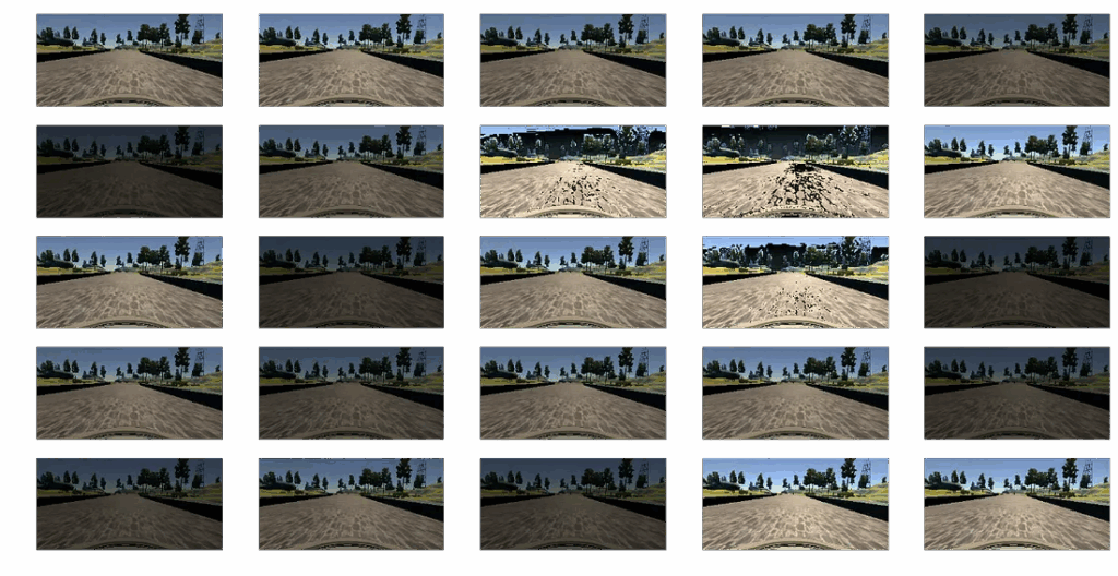
We have talked in great detail about object detection and segmentation, two of the main problems of computer vision. To solve them, models need training data, the more the merrier. In modern computer vision, training data is always in short supply, so researchers always use various data augmentation techniques to enlarge the dataset.
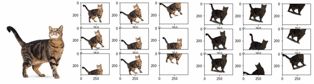
The point of data augmentation is to introduce various modifications of the original image that do not change the ground truth labels you have or change them in predictable ways. Common augmentation techniques include, for instance, moving and rotating the picture and changing its color histogram in predictable ways:
Notice how in terms of individual pixels, the pictures change completely, but we still have a very predictable and controllable transformation of what the result should be. If you know where the cat was in the original image, you know exactly where it is in the rotated-and-cropped one; and Instagram filters usually don’t change the labels at all.
Data augmentation is essential to reduce overfitting and effectively extend the dataset for free; it is usually silently understood in all modern computer vision applications and implemented in standard deep learning libraries (see, e.g., keras.preprocessing.image).
Cutting and pasting sounds like a wonderful idea in this regard: why not cut out objects from images and paste them onto different backgrounds? The problem, of course, is that it is hard to cut and paste an object in a natural way; we will return to this problem later in this post. However, last year (2017) has seen a few papers that claimed that you don’t really have to be terribly realistic to make the augmentation work.
The easiest and most straightforward approach was taken by Rao and Zhang in their paper “Cut and Paste: Generate Artificial Labels for Object Detection” (appeared on ICVIP 2017). They simply took an object detection dataset (VOC07 and VOC12), cut out objects according to their ground truth labels and pasted them onto images with different backgrounds. Like this:
Source: (Rao, Zhang, 2017)
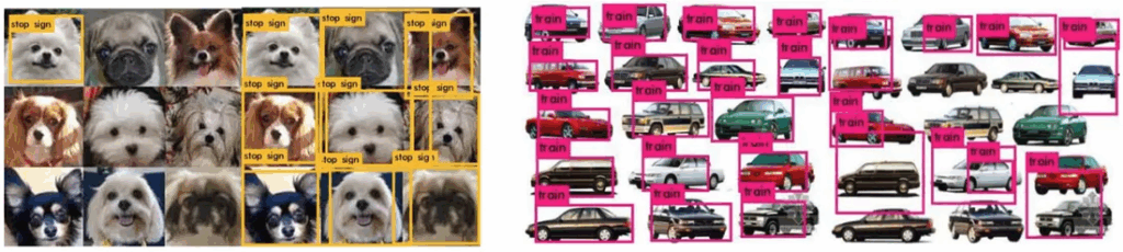
Then they trained with these images, using cut-and-paste like usual augmentation. Even with this very naive approach, they claimed to noticeably improve the results of standard object detection networks like YOLO and SSD. More importantly, they claimed to reduce common error modes of YOLO and SSD. The picture below shows the results after training on the left; and indeed, wrong labels decrease and bounding boxes significantly improve in many cases:
Source: (Rao, Zhang, 2017)
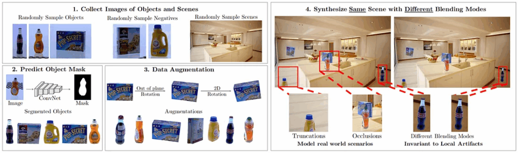
A similar but slightly less naive approach to cutting and pasting was introduced, also in 2017, by researchers from the Carnegie Mellon University. In “Cut, Paste and Learn: Surprisingly Easy Synthesis for Instance Detection” (ICCV 2017), Dwibedi et al. use the same basic idea but instead of just placing whole bounding boxes they go for segmentation masks. Here is a graphical overview of their approach:
Source: (Dwibedi et al., 2017)
Basically, they take a set of images of the objects they want to recognize, collect a set of background scenes, and then paste objects into the scene. Interestingly, they are recognizing grocery items in indoor environments, just like we did in our first big project on synthetic data.
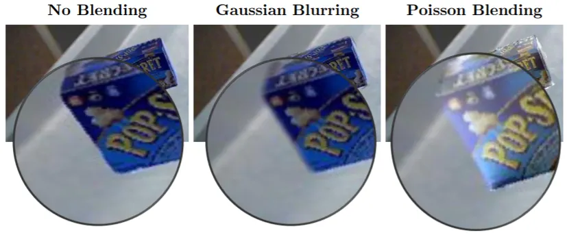
Dwibedi et al. claim that it is not really important to place objects in realistic ways globally but important to achieve local realism. That is, modern object detectors do not care as much to have a Coke bottle on the counter rather than on the floor; however, it is important to blend the object as realistically as possible into the local background. To this purpose, Dwibedi et al. consider several differ blending algorithms for pasting images:
Source: (Dwibedi et al., 2017)
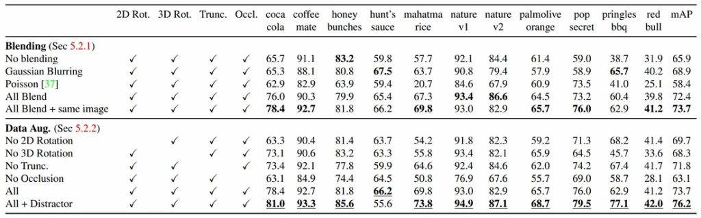
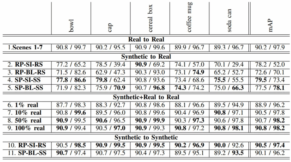
They then make blending another dimension of data augmentation, another factor of variability in order to make the detector robust against boundary artifacts. Together with other data augmentation techniques, it proves highly effective; “All Blend” in the table below means that all versions of blending for the same image are included in the training set:
Source: (Dwibedi et al., 2017)
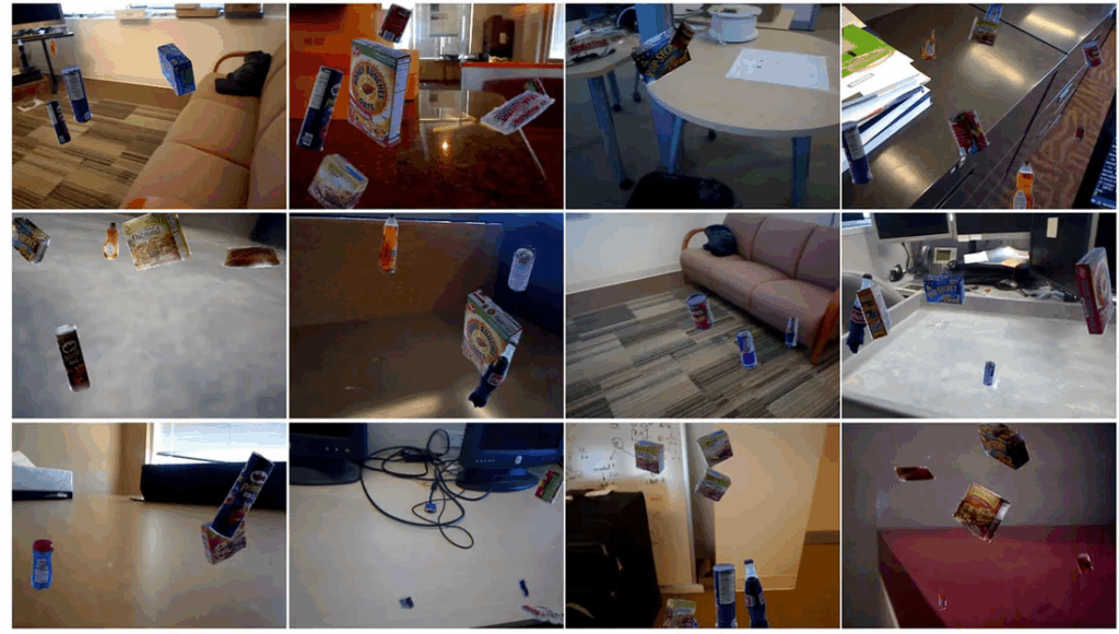
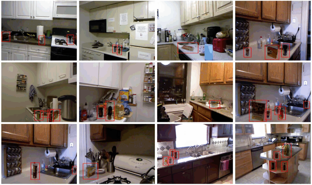
This also serves as evidence for the point about the importance of local realism. Here are some sample synthetic images Dwibedi et al. come up with:
Source: (Dwibedi et al., 2017)
As you can see, there is indeed little global realism here: objects are floating in the air with no regard to the underlying scene. However, here is how the accuracy improves when you go from real data to real+synthetic:
Source: (Dwibedi et al., 2017)
Note that all of these improvements have been achieved in a completely automated way. The only thing Dwibedi et al. need to make their synthetic dataset is a set of images for that would be easy to segment (in their case, they have photos of objects on a plain background). Then it is all in the hands of neural networks and algorithms: a convolutional network predicts segmentation masks, an algorithm does augmentation for the objects, and then blending algorithms make local patches more believable, so the entire pipeline is fully automated. Here is a general overview of what algorithms constitute this pipeline:
Source: (Dwibedi et al., 2017)
Smarter Augmentation: Pasting with Regard to Geometry
We have seen that even very naive pasting of objects can help improve object detection by making what is essentially synthetic data. The next step in this direction would be to actually try to make the pasted objects consistent with the geometry and other properties of the scene.
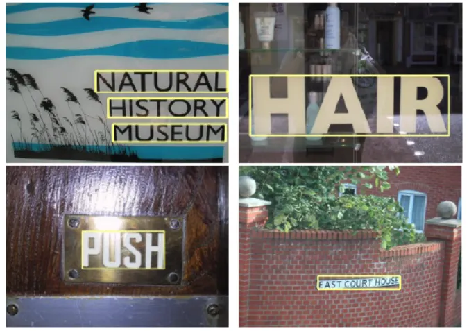
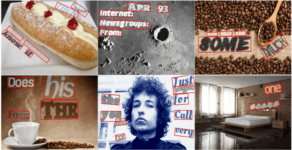
Here we begin with a special case: text localization, i.e., object detection specifically for text appearing on an image. That is, you want to take a picture with some text on it and output bounding boxes for the text instances regardless of their form, font, and color, like this:
This is a well-known problem that has been studied for decades, but here we won’t go into too many details on how to solve it. The point is, in 2016 (the oldest paper in this post, actually) researchers from the University of Oxford proposed an approach to blending synthetic text into real images in a way coherent with the geometry of the scene. In “Synthetic Data for Text Localisation in Natural Images”, Gupta et al. use a novel modification of a fully convolutional regression network (FCRN) to predict bounding boxes, but the main novelty lies in synthetic data generation.
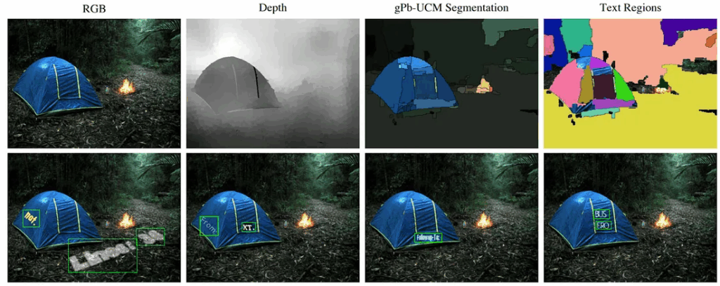
They first sample text and a background image (scraped from Google Image Search, actually). Then the image goes through several steps:
first, through a contour detection algorithm called gPb-UCM; proposed in (Arbelaez, Fowlkes, 2011), it does not contain any neural networks and is based on classical computer vision techniques (oriented gradient of histograms, multiscale cue combination, watershed transform etc.), so it is very fast to apply but still produces results that are sufficiently good for this application;
out of the resulting regions, Gupta et al. choose those that are sufficiently large and have sufficiently uniform textures: they are suitable for text placement;
to understand how to rotate the text, they estimate a depth map (with a state-of-the-art CNN), fit a planar facet to the region in question (with the RANSAC algorithm), and then add the text, blending it in with Poisson editing.
Here is a graphical overview of these steps, with sample generated images on the bottom:
Source: (Gupta et al., 2016)
As a result, Gupta et al. manage to produce very good text placement that blends in with the background scene; their images are not realistic only in the sense that we might not expect text to appear in these places at all, otherwise they are perfectly fine:
Source: (Gupta et al., 2016)
With this synthetic dataset, Gupta et al. report significantly improved results in text localization.
In “Synthesizing Training Data for Object Detection in Indoor Scenes”, Georgakis et al. from the George Mason University and University of North Carolina at Chapel Hill applied similar ideas to pasting objects into scenes rather than just text. Their emphasis is on blending the objects into scenes in a way consistent with the scene geometry and meaning. To do this, Georgakis et al.:
use the BigBIRD dataset (Big Berkeley Instance Recognition Dataset) that contains 600 different views for every object in the dataset; this lets the authors blend real images of various objects rather than do the 3D modeling required for a purely synthetic approach;
use an approach by Taylor & Cowley (2012) to parse the scene, which again uses the above-mentioned RANSAC algorithm (at some point, we really should start a NonNeuroNuggets series to explain some classical computer vision ideas — they are and will remain a very useful tool for a long time) to extract the planar surfaces from the indoor scene: counters, tables, floors and so on;
combine this extraction of supporting surfaces with a convolutional network by Mousavian et al. (2012) that combines semantic segmentation and depth estimation; semantic segmentation lets the model understand which surfaces are indeed supporting surfaces where objects can be placed;
then depth estimation and positioning of the extracted facets are combined to understand the proper scale and position of the objects on a given surface.
Here is an illustration of this process, which the authors call selective positioning:
Georgakis et al. train and compare Faster R-CNN and SSD with their synthetic dataset. Here is one of the final tables:
Source: (Georgakis et al., 2017)
We won’t go into the full details, but it basically shows that, as always, you can get excellent results on synthetic data by training on synthetic data, which is useless, and you don’t get good results on real data by training purely on this kind of synthetic data. But if you throw together real and synthetic then yes, there is a noticeable improvement compared to using just the real dataset. Since this is still just a form of augmentation and thus is basically free (provided that you have a dataset of different views of your objects), why not?
Cutting and Pasting for Segmentation… with GANs
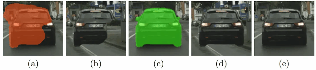
Finally, the last paper in our review is a quite different animal. In this paper recently released by Google, Remez et al. (2018) are actually solving the instance segmentation problem with cut-and-paste, but they are not trying to prepare a synthetic dataset to train a standard segmentation model. Rather, they are using cut-and-paste as an internal quality metric for segmentations: a good segmentation mask will produce a good image with a pasted object. In the image below, a bad mask (a) leads to an unconvincing image (b), and a good mask (c) produces a much better image (d), although the ground truth (e) is better still:
Source: (Remez et al., 2018)
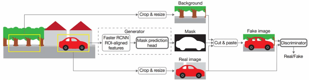
How does the model decide which images are “convincing”? With an adversarial architecture, of course! In the model pipeline shown below, the generator is actually doing the segmentation, and the discriminator judges how well the pasted image is by trying to distinguish it from real images:
Source: (Remez et al., 2018)
The idea is simple and brilliant: only a very good segmentation mask will result in a convincing fake, hence the generator learns to produce good masks… even without any labeled training data for segmentation! The whole pipeline only requires the bounding boxes for objects to cut out.
But you still have to paste objects intelligently. There are several important features required to make this idea work. Let’s go through them one by one.
1. Where do we paste? One can either paste uniformly at random points of the image or try to take into account the scene geometry and be smart about it, like in the papers above. Here, Remez et al. find that yes, pasting objects in a proper scale and place in the scene does help. And no wonder; in the picture below, first look on the left and see how long it takes you to spot the pasted objects. Then look on the right, where they have been pasted uniformly at random. Where will the discriminator’s job be easier?
Source: (Remez et al., 2018)
2. There are a couple of degenerate corner cases that formally represent a very good solution but are actually useless. For example, the generator could learn to “cut off” all or none of the pixels in the image and thus make the result indistinguishable from real… because it is real! To discourage from choosing all pixels, the discriminator simply receives a larger viewpoint, seeing, so to speak, the bigger picture, so this strategy ceases to work. To discourage from choosing no pixels, the authors introduce an additional classification network that attempts to classify the object of interest and the corresponding loss function. Now, if the object has not been cut, classification will certainly fail, incurring a large penalty.
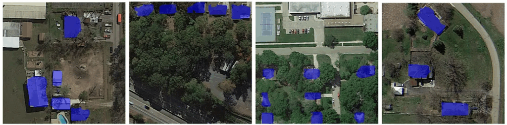
3. Sometimes, cutting only a part of the segmentation mask still results in a plausible object. This is characteristic for modular structures like buildings; for example, in these satellite images some of the masks are obviously incomplete but the resulting cutouts will serve just fine:
Source: (Remez et al., 2018)
To fix this, the authors set up another adversarial game, now trying to distinguish the background resulting from cutting out the object and the background resulting from the same cut elsewhere in the scene. This is basically yet another term in the loss function; modern GANs often tend to grow pretty complicated loss functions, and maybe someday we will explore them in more details.
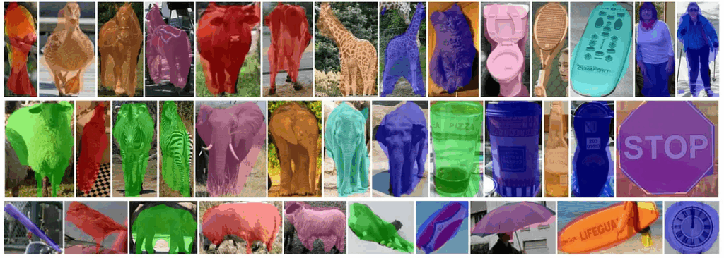
The authors compare their resulting strategy with some other pretrained baselines; while they, of course, lose to fully supervised methods (with access to ground truth segmentation masks in the training set), they come out ahead against the baselines. It is actually pretty cool that you can get segmentation masks like this with no effort for segmentation type labeling:
Source: (Remez et al., 2018)
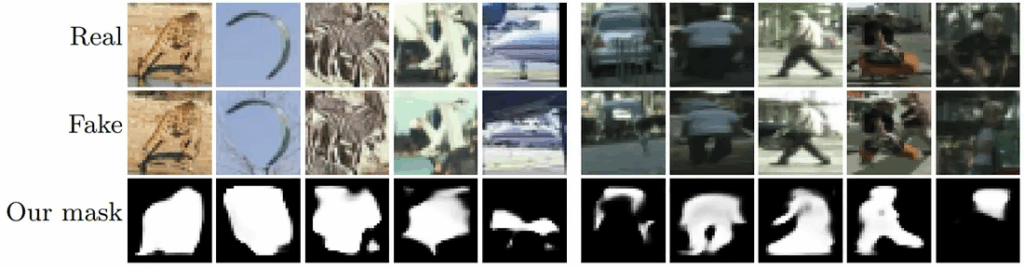
There are failure cases too, of course. Usually they happen when the result is still realistic enough even with the incorrect mask. Here are some characteristic examples:
Source: (Remez et al., 2018)
This work is a very interesting example of a growing trend towards data-independent methods in deep learning. More and more often, researchers find ways around the need to label huge datasets, and deep learning gradually learns to do away with the hardships of data labeling. We are not quite there yet but I hope that someday we will be. Until next time!
Sergey Nikolenko Chief Research Officer, Neuromation
I have said that she had no face; but that meant she had a thousand faces…
― C.S. Lewis, Till We Have Faces
Today we present to you another installment where we dive into the details about a few papers from the CVPR 2018 (Computer Vision and Pattern Recognition) conference. We’ve had four already: about GANs for computer vision, about pose estimation and tracking for humans, about synthetic data, and, finally, about domain adaptation. In particular, in the fourth part we presented three papers on the same topic that had actually numerically comparable results.
Today, we turn to a different problem that also warrants a detailed comparison. We will talk about face generation, that is, about synthesizing a realistic picture of a human face, either from scratch or by changing some features of a real photo. Actually, we already touched upon this problem a while ago, in our first post about GANs. But since then, generative adversarial networks (GANs) have been one of the very hottest topics in machine learning, and it is no wonder that new advances await us today. And again, it is my great pleasure to introduce Anastasia Gaydashenko with whom we have co-authored this text.
GANs for Face Synthesis and the Importance of Loss Functions
We have already spoken many times about how important a model’s architecture and a good dataset are for deep learning. In this post, one recurrent theme will be the meaning and importance of loss functions, that is, the functions that a neural network actually represents. One could argue that the loss function is a part of the architecture, but in practice we usually think about them separately; e.g., the same basic architecture could serve a wide variety of loss functions with only minor changes, and that is something we will see today.
We chose these particular papers because we liked them best, but also because they are all using GANs and are all using them to modify pictures of faces while preserving the person’s identity. This is a well-established application of GANs; classical papers such as ADD used it to predict how a person changes with age or how he or she would look like if they had a different gender. The papers that we consider today bring this line of research one step further, parceling out certain parts of a person’s appearance (e.g., makeup or emotions) in such a way that it can become subject to manipulations.
Thus, in a way all of today’s papers are also solving the same problem and might be comparable with each other. The problem, though, is that the true evaluation of a model’s results basically could be done only by a human: you need to judge how realistic the new picture looks like. And in our case, the specific tasks and datasets are somewhat different too, so we will not have a direct comparison of the results, but instead we will extract and compare new interesting ideas.
On to the papers!
Towards Open-Set Identity Preserving Face Synthesis
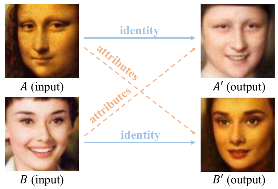
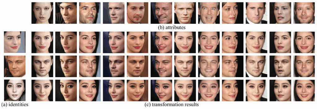
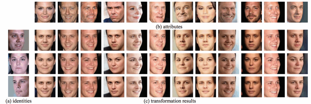
The authors of the first paper, a joint work of researchers from the University of Science and Technology of China and Microsoft Research (full pdf), aim to disentangle identity and attributes from a single face image. The idea is to decompose a face’s representation into “identity” and “attributes” in such a way that identity corresponds to the person, and attributes correspond to basically everything that could be modified while still preserving identity. Then, using this extracted identity, we can add attributes extracted from a different face. Like this:
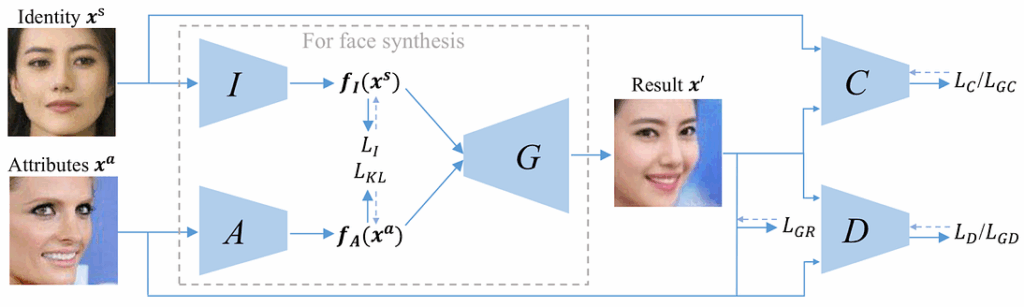
Fascinating, right? Let’s investigate how do they do it. There are quite a few novel interesting tricks in the paper, but the main contribution of this work is a new GAN-based architecture:
Here the network takes as input two pictures: the identity pictureand the attributes picture that will serve as the source for everything except the person’s identity: pose, emotion, illumination, and even the background.
The main components of this architecture include:
identity encoder I that produces a latent representation (embedding) of the identity input xˢ;
attributes encoder A that does the same for the attributes input xᵃ;
mixed picture generator G that takes as input both embeddings (concatenated) and produces the picture x’ that is supposed to mix the identity of xˢ and the attributes of xᵃ;
identity classifier C checks whether the person in the generated picture x’ is indeed the same as in xˢ;
discriminator D that tries to distinguish real and generated examples to improve generator performance, in the usual GAN fashion.
This is the structure of the model used for training; when all components have been trained, for generation itself it suffices to use only the part inside the dotted line, so the networks C and D are only included in the training phase.
The main problem, of course, is how to disentangle identity from attributes. How can we tell the network what it should take from xˢ and what from xᵃ? The architecture outlined above does not answer this question by itself, the main work here is done by a careful selection of loss functions. There are quite a few of them; let us review them one by one. The NeuroNugget format does not allow for too many formulas, so we will try to capture the meaning of each part of the loss function:
the most straightforward part is the softmax classification loss Lᵢ that trains identity encoder I to recognize the identity of people shown on the photos; basically, we train I to serve as a person classifier and then use the last layer of this network as features fᵢ(xs);
the reconstruction loss Lᵣ is more interesting; we would like the result x’ to reconstruct the original image xᵃ anyway but there are two distinct cases here:
if the person on image xᵃ is the same as on the identity image xs, there is no question what we should do: we should reconstruct xᵃ as exactly as possible;
and if xᵃ and xˢ show two different people (we know all identities on the supervised training phase), we also want to reconstruct xa but with a lower penalty for “errors” (10 times lower in the authors’ experiments); we don’t actually want to reconstruct xᵃ exactly now but still want x’ to be similar to xᵃ;
the KL divergence loss Lkl is intended to help the attributes encoder A concentrate on attributes and “lose” the identity as much as possible; it serves as a regularizer to make the attributes vector distribution similar to a predefined prior (standard Gaussian);
the discriminator loss Lᵈ is standard GAN business: it shows how well D can discriminate between real and fake images; however, there is a twist here as well: instead of just including discriminator loss Lᵈ the network starts by using Lᵍᵈ, a feature matching loss that measures how similar the features extracted by D on some intermediate level from x’ and xa are; this is due to the fact that we cannot expect to fool D right away, the discriminator will always be nearly perfect at the beginning of training, and we have to settle for a weaker loss function first (see the CVAE-GAN paper for more details);
and, again, the same trick works for the identity classifier C; we use the basic classification loss Lᶜ but also augment it with the distance Lᵍᶜ between feature representations of x’ and xˢ on some intermediate layer of C.
(Disclaimer: I apologize for slightly messing up notation from the pictures but Medium actually does not support sub/superscripts so I had to make do with existing Unicode symbols.)
That was quite a lot to take in, wasn’t it? Well, this is how modern GAN-based architectures usually work: their final loss function is usually a sum of many different terms, each with its own motivation and meaning. But the resulting architecture works out very nicely; we can now train it in several different ways:
first, networks I and C are doing basically the same thing, identifying people; therefore, they can share both the architecture and the weights (which simplifies training), and we can even use a standard pretrained person identification network as a very good initialization for I and C;
next, we train the whole thing on a dataset of images of people with known identities; as we have already mentioned, we can pick pairs of xˢ and xᵃ as different images of the same person and have the network try to reconstruct xa exactly, or pick xˢ and xᵃ with different people and train with a lower weight of the reconstruction loss;
but even that is not all; publicly available labeled datasets of people are not diverse enough to train the whole architecture end-to-end, but, fortunately, it even allows for unsupervised training; if we don’t know the identity we can’t train I and C, so we have to ignore their loss functions, but we can still train the rest! And we have already seen that I and C are the easiest to train, so we can assume they have been trained well enough on the supervised part. Thus, we can simply grab some random faces from the Web and add them to the training set without knowing the identities.
Thanks to the conscious and precise choice of the architecture, loss functions, and the training process, the results are fantastic! Here are two selections from the paper. In the first, we see transformations of faces randomly chosen from the training set with random faces for attributes:
And in the second, the identities never appeared in the training set! These are people completely unknown to the network (“zero-shot identities”, as the paper calls them)… and it still works just fine:
PairedCycleGAN: Asymmetric Style Transfer for Applying and Removing Makeup
This collaboration of researchers from Princeton, Berkeley, and Adobe (full pdf) works in the same vein as the previous paper but tackles a much more precise problem: can we add/modify the makeup on a photograph rather than all attributes at once, while keeping the face as recognizable as possible. A major problem here is, as it often happens in machine learning, with the data: a relatively direct approach would be quite possible if we had a large dataset of aligned photographs of faces with and without makeup… but of course we don’t. So how do we solve this?
The network still gets two images as an input: the source image from which we take the face and the reference image from which we take the makeup style. The model then produces the corresponding output; here are some sample results, and they are very impressive:
This unsupervised learning framework relies on a new model of a cycle-consistent generative adversarial network; it consists of the two asymmetric functions: the forward function encodes example-based style transfer, whereas the backward function removes the style. Here is how it works:
The picture shows two coupled networks designed to implement these functions: one that transfers makeup style (G) and another that can remove makeup (F); the idea is to make the output of their successive application to an input photo match the input.
Let us talk about losses again because they define the approach and capture the main new ideas in this work as well. The only notation we need for that is that X is the “no makeup” domain and Y is the domain of images with makeup. Now:
the discriminator DY tries to discriminate between real samples from domain Y (with makeup) and generated samples, and the generator G aims to fool it; so here we use an adversarial loss to constrain the results of G to look similar to makeup faces from domain Y;
the same loss function is used for F for the same reason: to encourage it to generate images indistinguishable from no-makeup faces sampled from domain X;
but these loss functions are not enough; they would simply let the generator reproduce the same picture as the reference without any constraints imposed by the source; to prevent this, we use the identity loss for the composition of G and F: if we apply makeup to a face x from X and then immediately remove it, we should get back the input image x exactly;
now we have made the output of G to belong to Y (faces with makeup) and preserve the identity, but we still are not really using the reference makeup style in any way; to transfer the style, we use two different style losses:
style reconstruction loss Ls says that if we transfer makeup from a face y to a face x with G(x,y), then remove makeup from y with F(y), and then apply the style from G(x,y) back to F(y), we should get y back, i.e., G(F(y), G(x,y)) should be similar to y;
and then on top of all this, we add another discriminator DS that decides whether a given pair of faces have the same makeup; its style discriminator loss LP is the final element of the objective function.
There is more to the paper than just loss functions. For example, another problem was how to acquire a dataset of photos for the training set. The authors found an interesting solution: use beauty-bloggers from YouTube! They collected a dataset from makeup tutorial videos (verified manually on Amazon Mechanical Turk), thus ensuring that it would contain a large variety of makeup styles in high resolution.
The results are, again, pretty impressive:
The results become especially impressive if you compare them with previous state of the art models for makeup transfer:
We have a feeling that the next Prisma might very well be lurking somewhere nearby…
Facial Expression Recognition by De-expression Residue Learning
With the last paper for today (full pdf), we turn from makeup to a different kind of very specific facial features: emotions. How can we disentangle identity and emotions?
In this work, the proposed architecture contains two learning processes: the first is learning to generate standard neutral faces by conditional GANs (cGAN), and the second is learning from the intermediate layers of the resulting generator. To train the cGANs, we use pairs of face images that show some expression (input), and a neutral face image of the same subject (output):
The cGAN is learned as usual: the generator reconstructs the output based on the input image, and then tuples (input, target, yes) and (input, output, no) are given to the discriminator. The discriminator tries to distinguish generated samples from the ground truth while the generator tries to not only confuse the discriminator but also generate an image as close to the target image as possible (composite loss functions again, but this time relatively simple).
The paper calls this process de-expression (removing expression from a face), and the idea is that during de-expression, information related to the actual emotions is still recorded as an expressive component in the intermediate layers of the generator. Thus, for the second learning process we fix the parameters of the generator, and the outputs of intermediate layers are combined and used as input for deep models that do facial expression classification. The overall architecture looks like this:
After neutral face generation, the expression information can be analyzed by comparing the neutral face and the query expression face at the pixel level or feature level. However, pixel-level difference is unreliable due to the variation between images (i.e., rotation, translation, or lighting). This can cause a large pixel-level difference even without any changes in the expression. The feature-level difference is also unstable, as the expression information may vary according to the identity information. Since the difference between the query image and the neutral image is recorded in the intermediate layers, the authors exploit the expressive component from the intermediate layers directly.
The following figure illustrates some samples of the de-expression residue, which are the expressive components for anger, disgust, fear, happiness, sadness, and surprise respectively; the pictures shows the corresponding histogram for each expressive component. As we can see, both expressive components and corresponding histograms are quite distinguishable:
And here are some sample results on different datasets. In all pictures, the first column is the input image, the third column is the ground-truth neutral face image of the same subject, and the middle is the output of the generative model:
As a result, the authors both get a nice network for de-expression, i.e., removing emotion from a face, and improve state of the art results for emotion recognition by training the emotion classifier on rich features captured by the de-expression network.
Final words
Thank you for reading! With this, we are finally done with CVPR 2018. It is hard to do justice to a conference this large; naturally, there were hundreds of very interesting papers that we have not been able to cover. But still, we hope it has been an interesting and useful selection. We will see you again soon in the next NeuroNugget installments. Good luck!
Sergey Nikolenko Chief Research Officer, Neuromation
Anastasia Gaydashenko former Research Intern at Neuromation, currently Machine Learning Intern at Cisco
We have already had three installments about the CVPR 2018 (Computer Vision and Pattern Recognition) conference: the first part was devoted to GANs for computer vision, the second part dealt with papers about recognizing human beings (pose estimation and tracking), and the third part tackled synthetic data. Today we dive deeper into the details of one field of deep learning that has been on the rise lately: domain adaptation. For this NeuroNugget, I’m happy to present to you my co-author Anastasia Gaydashenko, who has already left Neuromation and went on to join Cisco…but her texts live on, and this is one of them.
What is Domain Adaptation?
There are a couple of specific directions in research that are trending lately (including CVPR 2018), and one of them is domain adaptation. As this field is closely related to synthetic data, it is of great interest for us here at Neuromation, but the topic is also increasingly popular and important in and by itself.
Let’s start at the beginning. We have already discussed the most common tasks that constitute the basis for modern computer vision: image classification, object and pose detection, instance and semantic segmentation, object tracking, and so on. These problems are solved quite successfully due to deep convolutional neural architectures and large amounts of labeled data.
But, as we discussed in the last installment, a big challenge always remains: for supervised learning, you always need to find or create labeled datasets. Almost any paper you read about some fancy state of the art model will mention some problems with the dataset, unless they use one of the few standard “vanilla” datasets that everybody usually compares on. Thus, collecting labeled data has become as important as designing the networks themselves. These datasets should be reliable and diverse enough so researchers would be able to use them to develop and evaluate novel architectures.
We have already talked many times about how manual data collection is both expensive and time-consuming, often exceedingly so. Sometimes it is even flat out impossible to label the data manually (for example, how do you label for depth estimation, the problem of evaluating the distances from points on the image to the camera?). Of course, many standard problems already have large labeled datasets that are freely or easily available. But first, this readily labeled data can (and does) bias research towards the specific field where it is available, and second, your own problem will never be exactly the same, and standard datasets will often simply not fit your demands: they will contain different classes, will be biased in different ways, and so on.
The main problem with using existing datasets, or even synthetic data generators that were not done specifically for your particular problem, is that when the data is generated and already labeled we are still facing the problem of domain transfer: how do we use one kind of data to prepare the networks to cope with different kinds? This problem also looms large for the entire field of synthetic data: however realistic you make your data, it still cannot be completely indistinguishable from real world photographs. The major underlying challenge here is known as domain shift: basically, the distribution of data in the target domain (say, real images) is different than in the source domain (say, synthetic images). Devising models that can cope with this shift is exactly the problem called domain adaptation.
Let us see how people are handling this problem now, considering a few papers from CVPR 2018 in slightly more details than we used to in previous “CVPR in Review” installments.
Unsupervised Domain Adaptation with Similarity Learning
This work by Pedro Pinheiro (see pdf here) comes from ElementAI, a Montreal company co-founded in 2016 by none other than Yoshua Bengio. It deals with an approach to domain adaptation based on adversarial networks, the kind we touched upon a little bit before (see also this post, the second part for which is coming really soon… it is, it is, I promise!).
The simplest adversarial approach to unsupervised domain adaptation is a network that tries to extract features that remain the same across the domains. To achieve this, the network tries to make them indistinguishable for a separate part of the network, a discriminator (“disc” in the figure below). But at the same time, these features should be representative for the source domain so the network will be able to classify objects:
In this way, the network has to extract features that would achieve two objectives at once: (1) be informative enough that the “class” network (usually very simple) can classify, and (2) be independent of the domain so that the “disc” network (usually as complex as the feature extractor itself, or more) cannot really distinguish. Note that we don’t have to have any labels for the target domain, only for the source domain, where it is usually much easier (again, think synthetic data for the source domain).
In Pinheiro’s paper, this approach is improved by replacing the classifier part with a similarity-based one. The discriminative part remains the same, and the classification part now compares the embedding of an image with a set of prototypes; all these representations are learned jointly and in an end-to-end fashion:
Basically, we are asking one network, g, to extract features from a labeled source domain and another network, f, to extract features from an unlabeled target domain, with a similar but different data distribution. The difference is that now f and g are different (we had the same f in the picture above), and the classification is now different: instead of training a classifier, we train the model to discriminate the target prototype from all other prototypes. And to label the image from the target domain, we compare the embedding of an image with embeddings of prototype images from the source domain, assigning the label of its nearest neighbors:
The paper shows that the proposed similarity-based classification approach is more robust to the domain shift between the two datasets.
Image to Image Translation for Domain Adaptation
In this work by Murez et al. (full pdf), coming from UCSD and HRL Laboratories, the main idea is actually rather simple, but the implementation is novel and interesting. The work deals with a more complex task than classification, namely image segmentation (see, e.g., our previous post), which is widely used in autonomous driving, medical imaging, and many other domains. So what is this “image translation” thing they are talking about?
Let us begin with regular translation. Imagine that we have two large text corpora in different languages, say English and French, and we don’t know which phrases correspond to which. They may be even slightly different and may lack the corresponding translations in the other language corpus. Just like the pictures from synthetic and real domains. Now, to get a machine translation model we translate a phrase from English to French and will try to distinguish the embedding of the resulting phrase from embeddings of phrases from the original French corpus. And then the way to check that we haven’t lost much is to try to translate this phrase back to English; now, even if the original corpora were completely unaligned, we know what we’re looking for: the answer is just the original sentence!
Now let us look at the image to image translation which is, actually, pretty similar. Basically, domain adaptation techniques aim to address the domain shift problem by finding a mapping from the source data distribution to the target distribution. Alternatively, both domains X and Y could be mapped into a shared domain Z where the distributions are aligned; this is the approach used in this paper. This embedding must be domain-agnostic (independent of the domain), hence we want to maximize the similarity between the distributions of embedded source and target images.
For example, suppose that X is the domain of driving scenes on a sunny day and Y is the domain of driving scenes on a rainy day. While “sunny” and “rainy” are characteristics of the source and target domains, they are in fact variations that mean next to nothing for the annotation task (e.g., semantic segmentation of the road), and they should not affect the annotations. Treating such characteristics as structured noise, we would like to find a latent space Z that would be invariant to such variations. In other words, domain Z should not contain domain-specific characteristics, that is, be domain-agnostic.
In this case, we also want to restore annotations for an image from the target domain. Therefore, we also need to add a mapping from the shared embedding space to the labels. It may be image-level labels such as classes in a classification problem or pixel-level labels such as semantic segmentation:
Basically, that’s the whole idea! Now, to obtain the annotation for an image from the target domain we just need to get its embedding in the shared space Z and restore its annotation from C. This is the basic idea of the approach, but it can be further improved by the ideas proposed in this paper.
Specifically, there are three main tools needed to achieve successful unsupervised domain adaptation:
domain-agnostic feature extraction, which means that distributions of features extracted from both domains should be indistinguishable as judged by an adversarial discriminator network,
domain-specific reconstruction, which means that we should be able to decode embeddings back to the source and target domains, that is, we should be able to learn functions gX and gY like shown here:
cycle consistency to ensure that the mappings are learned correctly, that is, we should be able to get back where we started in cycles like this:
The whole point of the framework proposed in this work is to ensure these properties with loss functions and adversarial constructions. We will not go into the gritty details of the architectures since they may change for other domains and problems.
But let’s have a look at the results! At the end of the post, we will make a detailed comparison between three papers on domain adaptation, but now let’s just have a look at a single example. The paper used two datasets: a synthetic dataset from Grand Theft Auto 5 and a real-world Cityscapes dataset with pictures of cities. Here are two sample pictures:
And here are the segmentation results for the real-world image (B above):
On this picture, E is the ground truth segmentation, C is the result produced without domain adaptation, simply by training on the synthetic GTA5 dataset, and D is the result with domain adaptation. It does look better, and the numbers (intersection-over-union metric) do bear this out.
Conditional Generative Adversarial Network for Structured Domain Adaptation
This paper by Hong et al. (full pdf) proposes another modification of a standard discriminator-segmentator architecture. From the first look at the architecture, we may not even notice any difference:
But actually this architecture does something very interesting: it integrates a GAN into a fully convolutional network (FCN). We have discussed FCNs in a previous NeuroNugget post; it s the network architecture used for the segmentation problem that returns labels for each pixel in the picture by feeding the features through deconvolution layers.
In this model, a GAN is used to mitigate the gap between source and target domains. For example, the previous paper aligns two domains via an intermediate feature space and thereby implicitly assumes the same decision function for both domains. This approach relaxes this assumption: here we learn the residual between feature maps from both domains because the generator learns to produce features like the ones from a real image in order to fool the discriminator; afterwards,FCN parameters are updated to accommodate the changes GAN has made.
Again, we will show a numerical comparison of the result below but here are some examples from the dataset:
Remarkably, in this work the authors have also provided something very similar to what we are doing in our studies into the efficiency of synthetic data: they have measured the accuracy of the results (again measured with intersection-over-union) depending on the portion of synthetic images in the dataset:
Learning from Synthetic Data: Addressing Domain Shift for Semantic Segmentation
This work by Sankaranarayanan et al. (full pdf) presents another modification of the basic approach based on GANs that brings the embeddings closer in the learned feature space. This time, let us begin with the picture and then explain it:
The base network, whose architecture is similar to a pre-trained model such as VGG-16, is split into two parts: the embedding denoted by F and the pixel-wise classifier denoted by C. The output of C is a map of labels upsampled to the same size as the input of F. The generator network G takes as input the learned embedding and reconstructs the RGB image. The discriminator network D performs two different tasks given an input: it classifies the input as real or fake in a domain-consistent manner and also performs a pixel-wise labeling task similar to the network C (this is applied only to source data since target data does not come with any labels during training).
So the main contribution of this work is a technique that employs generative models to align the source and target distributions in the feature space. For this purpose, the authors first project intermediate feature representations obtained using a CNN to the image space by training a reconstruction part of the network and then impose the domain alignment constraint by forcing the network to learn features such that source features produce target-like images when passed to the reconstruction module and vice versa.
Sounds complicated, doesn’t it? Well, let’s see how all of these methods actually compare.
A Numerical Comparison of the Results
We have chosen these three papers for an in-depth look because their results are actually comparable! All three papers used domain adaptation with GTA5 as the source (synthetic) dataset and Cityscapes as the target dataset, so we can literally just compare the numbers.
The Cityscapes dataset contains 19 classes characteristic for city outdoor scenes such as “road”, “wall”, “person”, “car”, etc. And all three papers actually contain tables with results broken down with respect to the classes.
Murez et al., image-to-image translation:
Hong et al., conditional GAN:
Sankaranarayanan et al., GAN in an FCN:
The mean results are 31.8, 44.5, 37.1 respectively, so it appears that the image-to-image approach is the least successful and Conditional GAN is the winner. For clarity, let us also compare the top-3 most and least distinguishable classes (i.e., with best and worst results) for every approach.
Most distinguishable, in the same order of models:
road (85.3), car (76.7), veg (72.0)
road (89.2), veg (77.9), car (77.8)
road (88.0), car (80.4), veg (78.7)
This is not too interesting, obviously roads and cars are always the best. But with the worst classes the situation is different:
train (0.3), bike (0.6), rider (3.3)
train (0.0), fence (10.9), wall (13.5)
train (0.9), t sign (11.6), pole (16.7)
Again, the “train” class seems to pose some kind of an insurmountable challenge (probably there’re just not so many trains in the training set, pardon the pun), but the others are all different. So let us compare all models based on the “bike”, “rider”, “fence”, “wall”, “t sign”, and “pole” classes. Now their scores will be very distinct:
You can draw different conclusions from these results. But the main result that we personally find truly exciting is that with many different approaches that could be proposed for such a complex task, results in different papers at the same conference (so the authors could not follow one another, these results appeared independently) are perfectly comparable with each other, and researchers do not hesitate to publish these comparable numbers instead of some comfortable self-developed metrics that would prove their unquestionable supremacy. Way to go, modern machine learning!
And finally, let us finish on a lighter note, with one more fun paper about synthetic data.
Free supervision from video games
In this work, Philipp Krähenbühl (full pdf) created a wrapper for the ever popular Microsoft DirectX rendering API and added a specialized code into the game as it is running. This enables the DirectX engine to produce ground truth labels for instance segmentation, semantic labeling, depth estimation, optical flow, intrinsic image decomposition, and instance tracking in real time! Which sounds super cool because now, instead of labeling data manually or creating special purpose synthetic data engines, a researcher can just play video games all day long! All you need to do is find a suitable 3D game:
And with that, we finish the fourth installment on CVPR 2018. Thank you for your attention — and stay tuned!
Sergey Nikolenko Chief Research Officer, Neuromation
Anastasia Gaydashenko former Research Intern at Neuromation, currently Machine Learning Intern at Cisco
The CVPR 2018 (Computer Vision and Pattern Recognition) conference is long over, but we can’t stop reviewing its wonderful papers; today, Part III is upon us! In the first part, we briefly reviewed the most interesting papers on GANs for computer vision from CVPR 2018; in the second part, added a human touch and talked about pose estimation and tracking for humans. Today, we turn to one of the main focal point of our own internal research here at Neuromation: synthetic data. As usual, the papers are in no particular order, and our reviews are very brief, so we definitely recommend to read the papers in full.
Synthetic data: imitate to learn
Synthetic data means data that has been generated artificially, either through 3D modeling and rendering (as usual for computer vision) or by other means, and then used to train machine learning models. Synthetic data is a surprising topic in machine learning, and the most surprising thing is for how long it had been mostly neglected. Some works on synthetic data can be traced to the 2000s, but before 2016 it basically attracted no interest at all. The only field where it had been used was to train self-driving cars, where the need for simulated environments and the impossibility to collect real datasets come together and make it the perfect situation for synthetic datasets.
Now the interest is rapidly growing: we now have the SUNCG dataset of simulated indoor environments, outdoor environments for driving and navigation, the SURREAL dataset of synthetic humans to learn pose estimation and tracking, and even recent works that apply GANsto generate and refine synthetic data (we hope to get back to this and explain how it works later). So let us see what CVPR 2018 authors have to say about synthetic data. Since this is our main focus, we will consider the works on synthetic data in slightly more detail than usual.
Generating Synthetic Data from GANs: Augmentation and Adaptation in Feature Space
There is a very interesting and promising field of using GANs to produce synthetic datasets to train other models. On the surface it makes little sense: if you have enough data to train a GAN, why not just use it to train the model? Or even better, if you have a trained GAN why don’t you just take the discriminator and use it for your problem?
But this idea becomes much more interesting in the domain adaptation setting. Suppose you have a large source dataset and a small target dataset, and you need to use a model trained on the source dataset for the target, which might be completely unlabeled. Here adversarial domain adaptation techniques train two networks, a generator and a discriminator, and use it to ensure that the network cannot distingush between the data distributions in the source and target datasets. This field was started in the ICML 2015 paper by Ganin and Lempitsky, where the discriminator is used to ensure that the features stay domain-invariant:
In the CVPR 2018 paper by Volpi et al., researchers from Italy and Stanford made the adversarial training work not on the original images but rather in the feature space itself. The GAN operated on features extracted by a pretrained network, which makes it possible to achieve better domain invariance and ultimately improve the quality of domain adaptation. Here is the overall training procedure as it was adapted by Volpi et al.:
Another approach in the same vein was presented in CVPR 2018 by Sankaranarayanan et al., researchers from the University of Maryland. They use GANs to leverage unsupervised data to bring the source and target distributions closer to each other in the feature space. Basically, the idea is to use the discriminator to control that images generated from an embedding remain realistic images for the source distribution even when the embedding was taken from a sample from the target distribution. Here is how it works, and, again, the authors report improved domain adaptation results:
How Well Should You Label? A Study of Label Quality
One of the main selling points of synthetic data has always been the pixel-perfect quality of labeling that you can easily achieve with synthetic data. A synthetic scene always comes with perfect segmentation — but just how important is it? The authors of this work studied how fine (or how coarsely) you have to label your training set to get good segmentation quality from modern convolutional architectures… and, of course, what better tool to perform this study than synthetic scenes.
The authors used their specially developed Auto City dataset:
And in their experiments, the authors showed that the final segmentation quality, unsurprisingly, is indeed strongly correlated with the amount of time spent to produce the labels… but not so much with the quality of each individual label. This suggests that it is better to produce lots of coarse labels (say, with crowdsourcing) than to perform strict quality control for every label.
Here at Neuromation, we love soccer (yes, the World Cup in Russia cost us a lot of work hours), and this research is just soooooooo cool. The authors present a system that can take a video stream of a soccer game and transform it… into a moving 3D reconstruction that can be projected onto your tabletop and viewed with an augmented reality device!
The system extracts bounding boxes of the players, analyzes the human figures with pose and depth estimation models and produces a quite accurate 3D scene reconstruction. Note how training a model specifically for the soccer domain really improves the results:
It additionally warms our hearts that they actually trained on synthetic data extracted from FIFA games! And the results are simply very cool all around:
But wait, there is more…
Thank you for your attention! Next time we might take an even more detailed look at some of the CVPR 2018 papers regarding synthetic data and domain adaptation. Until then!
Sergey Nikolenko Chief Research Officer, Neuromation