Today, I continue the series on synthetic data for object detection. In the first post of the series, we discussed the object detection problem itself and real world datasets for it, and the second was devoted to popular synthetic datasets of common objects. The time has come to put this data in practice: in this and subsequent posts, we will discuss common contemporary object detection architectures and see how adding synthetic data fares for object detection as reported in literature. In each post, I will give a detailed account of one paper that stands out in my opinion and briefly review one or two more. We begin in 2015.

Learning Deep Object Detectors from 3D Models
Here at Synthesis AI, we are making synthetic data for all kinds of models, but we are personally most interested in deep learning. In particular, object detection and segmentation have been overrun by deep neural networks over the last several years, and before people come up with something completely different it’s hard to imagine going back to classical computer vision.
Therefore, my story of synthetic data for object detection could not begin earlier than the first deep learning models for this problem… but it does not begin much later either! Our first paper in this review is by Peng et al., called “Learning Deep Object Detectors from 3D Models”; it came out on ICLR 2015, and the preprint is dated 2014.
So what was the state of the art in object detection back in 2014? The deep learning revolution in computer vision was still in early stages, so in terms of image classification architectures that could serve as backbones for object detection we had AlexNet, VGG, and GoogLeNet (the first in the Inception line). But at the time, there was little talk about “backbones”: the state of the art in object detection, reporting a huge improvement over the ILSVRC2013 detection track winner OverFeat (31.4% mIoU vs. 24.3% for OverFeat) was R-CNN by Girshick et al. (2013).
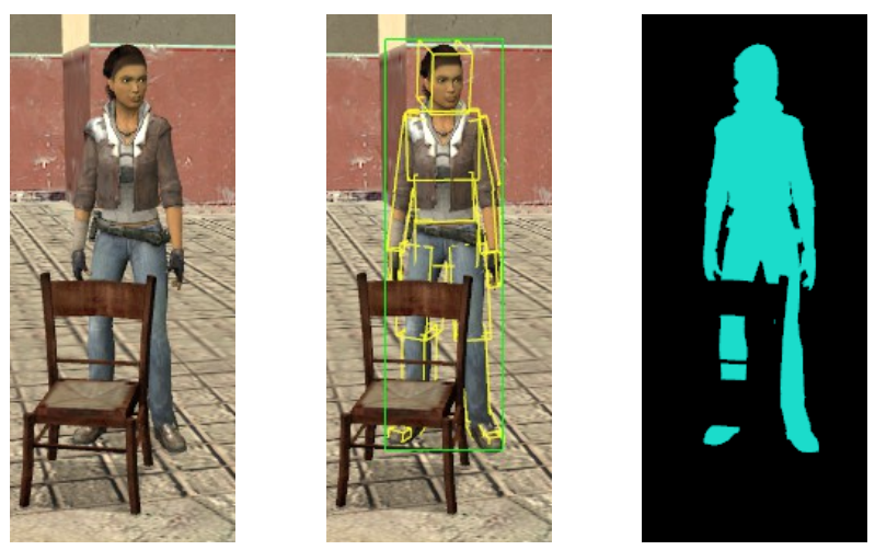
R-CNN is the most straightforward two-stage object detection architecture you can think of: bounding box proposals are produced by an external algorithm (the staple of the era, selective search by Uijlings et al.), and then each proposal goes through a convolutional network (CNN) for classification, with a separate model confirming whether the proposal actually does contain an object (because algorithms like selective search always produce a lot of false positives before you can be sure the real objects are covered). Like this:
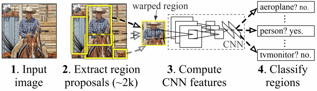
R-CNN was hopelessly slow (it took up to a minute to process a single picture!), but later it was sped up by incorporating all elements of the pipeline (bounding box proposal and evaluation) into the neural architecture. The result, Faster R-CNN, became a staple of two-stage object detection architectures, quite relevant even today.
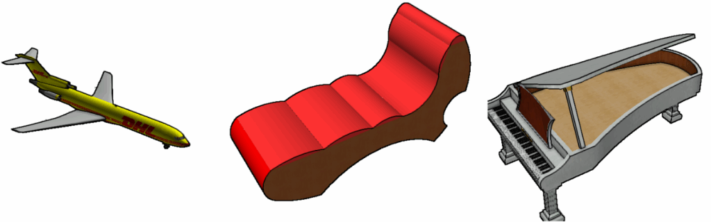
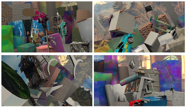
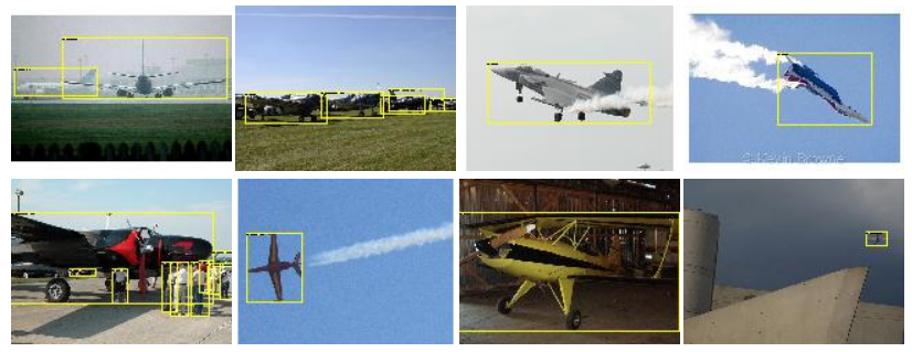
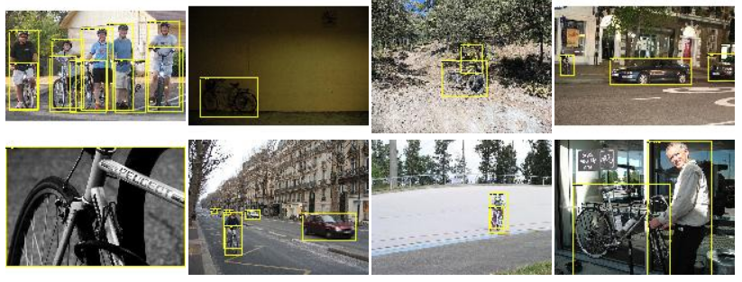
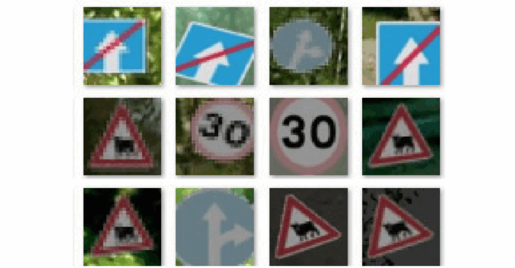
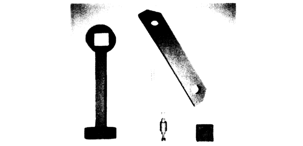
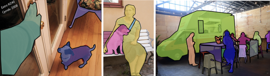
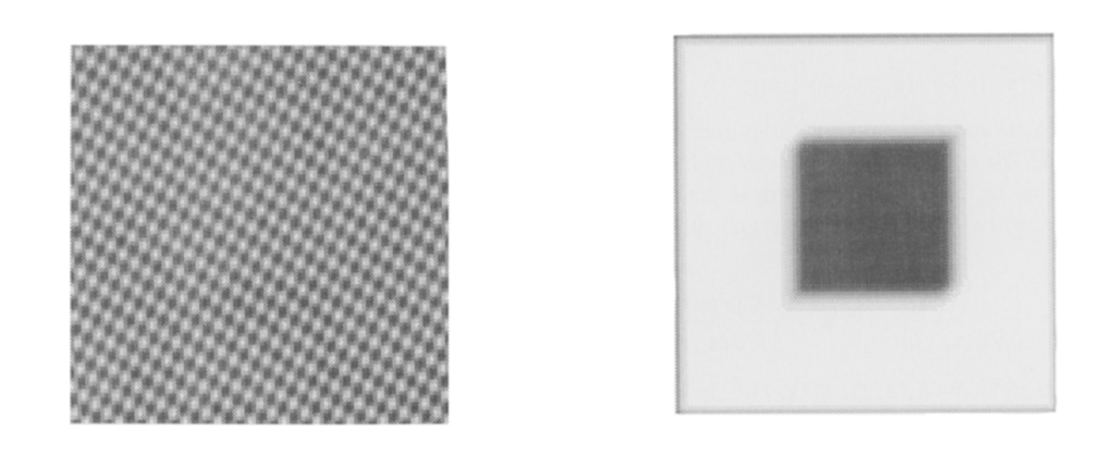
Back in 2014, researchers were still not sure if synthetic data was helpful. Moreover, the synthetic data they had was far from photorealistic, it was more like the ShapeNet dataset we discussed in a previous post. The work by Peng et al. was in many ways intended to study this very question: can you improve object detection or, say, learn to recognize new categories with synthetic data that looks like this:
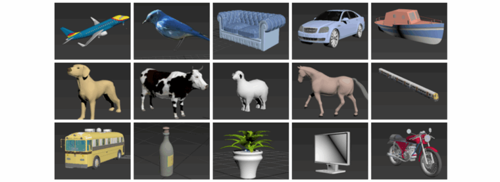
Thus, the main question for Peng et al. was to separate different “visual cues”, i.e., different components of an object. Simplistic synthetic data does pretty well in terms of shape, but poorly in terms of texture or realistic varied poses, and the background will have to be inserted separately so it probably won’t match too well. Given this discrepancy in quality, what can we expect from object detection models?
To study this question, Peng et al. propose an object detection pipeline that looks like R-CNN but is actually even simpler than that:
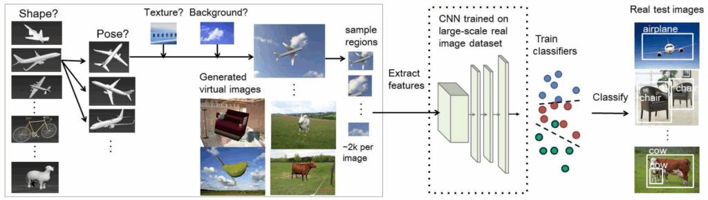
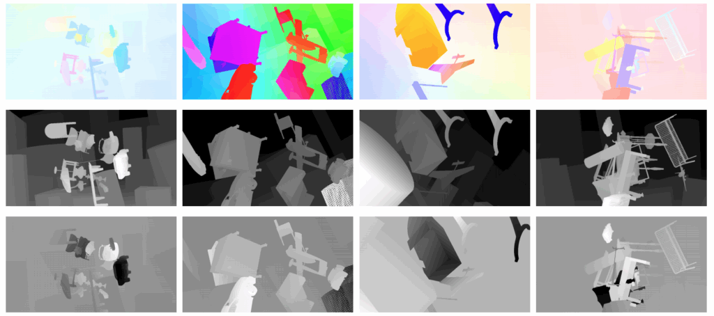
They used AlexNet pretrained on ImageNet as a feature extractor, and trained classifiers on features extracted from region proposals, just like R-CNN. Then they started testing for robustness to various cues, producing different synthetic datasets and testing object detection performance on a real test set after training on these datasets. Here is a sample table of results from their paper.
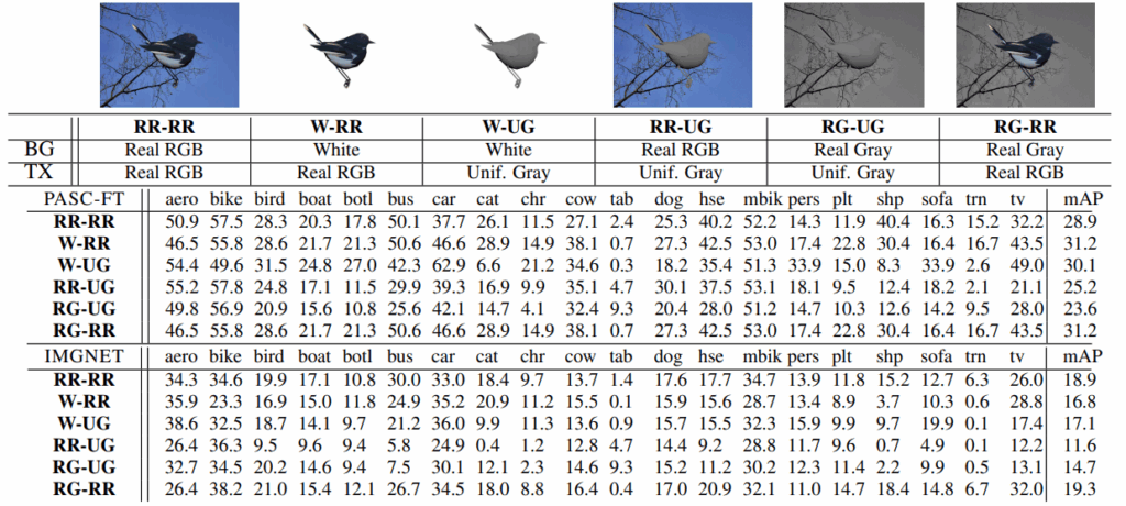
What do we see in this table? Well, interestingly, the results do not follow the standard intuition that the more details you have, the better the results will be. The simplest synthetic data, the W-UG row with uniform gray objects on white backgrounds, yields very reasonable results and significantly outperforms gray objects on more complex backgrounds.
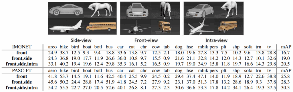
On the other hand, experiments by Peng et al. show that adding a more varied set of views for a given object always helps, sometimes significantly. In the tables below, adding another view for synthetic shapes leads to improvements in the final quality on real test datasets.
The absolute numbers in these tables did not really represent state of the art in object detection even in 2015, and are definitely not relevant today. But conclusions and comparisons show an important trend that goes through many early results on synthetic data for computer vision: for many models, the details and textures don’t matter as much since the models are looking for shapes and object boundaries. If that is the case for your model, then it is much more important to have a variety of shapes and poses, and textures can be left as an afterthought.
By now, I would probably generalize this lesson: different cues may be of different importance to different models. So unless you are willing to invest some serious resources into making an effort to achieve photorealism across the board, experiment with your model and find out what aspects are really important and worth investing for, and what aspects can be neglected (e.g., in this case you can leave the objects gray and skip the textures). This is what Peng et al. teaches us, and I believe it is as relevant in 2020 as it was in 2015.
First Attempts at Synthetic Videos for Object Detection
This was the detailed part, and for a brief review today let us consider one of the first attempts to use synthetic videos for object detection by Bochinski et al. (2016), in a work called “Training a convolutional neural network for multi-class object detection using solely virtual world data“. This is one of the first attempts I could find at building a complete virtual world with the intent of making synthetic data for computer vision systems, and specifically for object detection.
Bochinski et al. were also among the pioneers in using game engines for synthetic data generation. As the engine, they used Garry’s Mod, a sandbox game on the Source engine designed by Valve for Half Life and Counter Strike. Released in 2004 as a Half Life 2 mod intended to showcase the capabilities of the Source engine, Garry’s Mod remains a popular game even today; I saw it among my Steam recommendations less than a month ago…
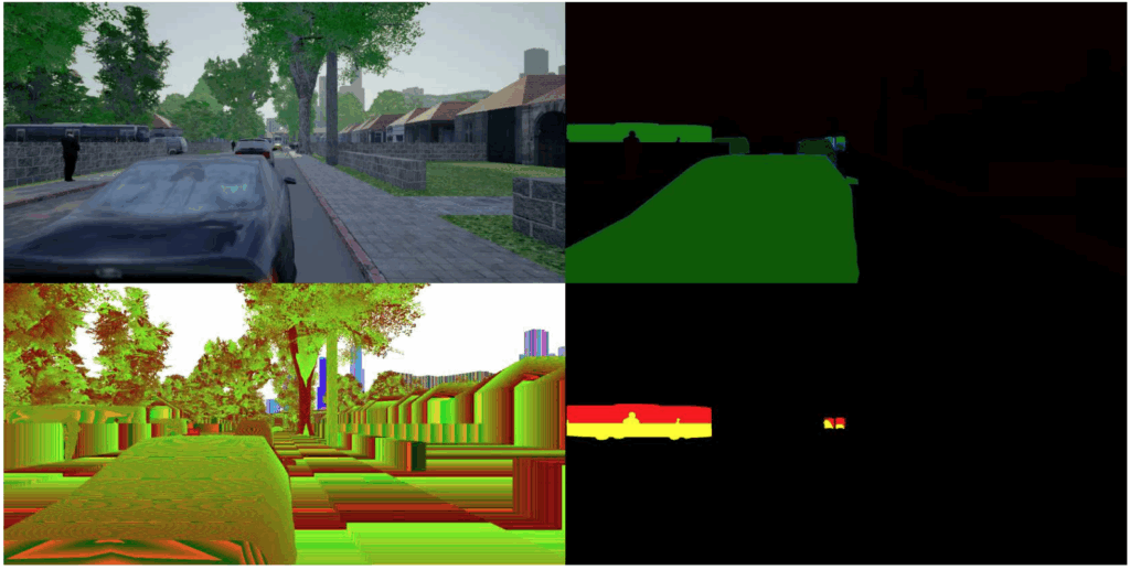
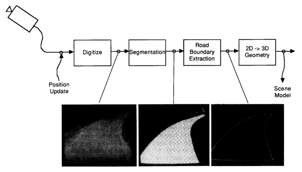
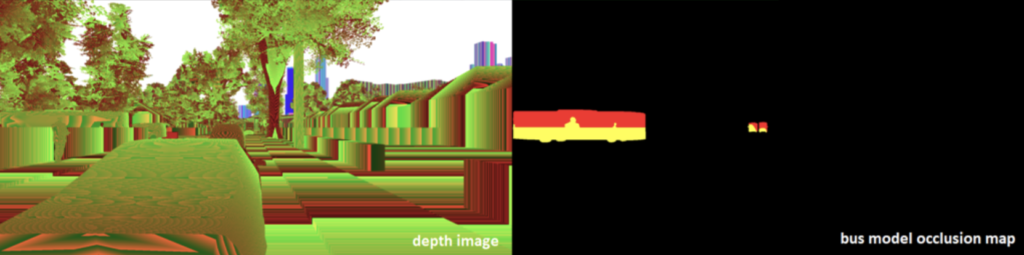
Anyway, the point of both Garry’s Mod and its use in Bochinski et al. is that Source has a very capable physics engine, and even more than that, it supports scripting for bots, both human and vehicles. Thus, it is relatively easy to create a simulated world for urban driving applications, complete with humans, cars, and surveillance cameras placed in realistic positions. Bochinski et al. extended the engine to be able to export bounding boxes, segmentation, and other kinds of labeling:
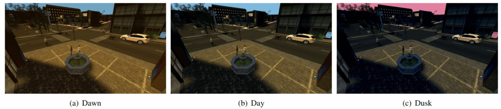
As for the rest, the Source engine allows to vary lighting conditions and, naturally, place cameras at arbitrary positions, e.g., in realistic surveillance camera locations:
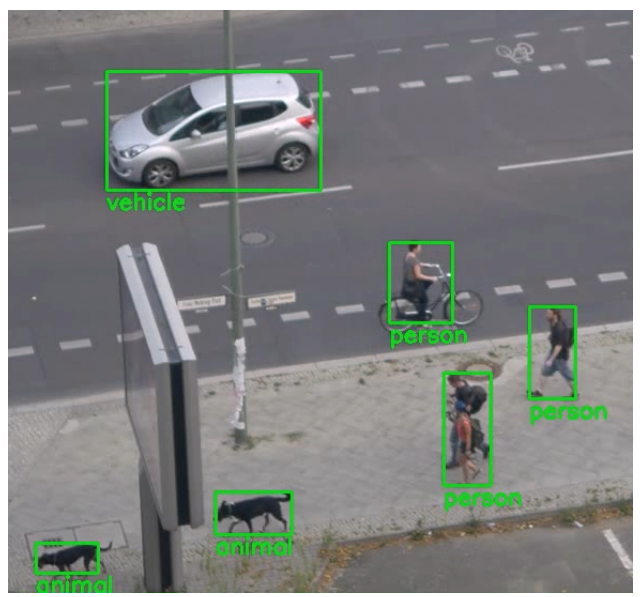
For object detection, since Bochinski et al. work with video data, they used a simple classical technique to construct bounding boxes: background subtraction. Basically, this means that they train a Gaussian mixture model to describe the history of every pixel, and if the pixel becomes different enough, it is considered to be part of the foreground (an object) rather than background. CNNs are only used (and trained) to do classification in the resulting bounding boxes. As a result, they achieve pretty good results even on a real test set:
So what’s the takeaway? This paper exemplifies how synthetic data can be helpful even for outdated pipelines: here, the bounding boxes were detected with a classical algorithm, so synthetic data was only used to train the classifier, and it still helped and resulted in a reasonable surveillance application.
Conclusion
Today, we have begun our account of synthetic data used to improve object detection pipelines. In fact, it is not easy to find papers that concentrate on object detection: since with synthetic data you can get any kind of labeling for free, most works skip right to segmentation or even more complex 3D-related problems. We have discussed two relatively early works (from 2015 and 2016) that, I believe, have something to tell us even today.
The main takeaway point is, in my opinion, this: different models may prove to be robust to the (un)realism of different aspects of synthetic data. This means that in practice, when you develop a synthetic dataset for an existing model or class of models for a given problem, it often pays to produce an ablation study and find out where you need to invest the most effort. Next time, we will move on to multiple object detection in constrained spaces — stay tuned!
Sergey Nikolenko
Head of AI, Synthesis AI