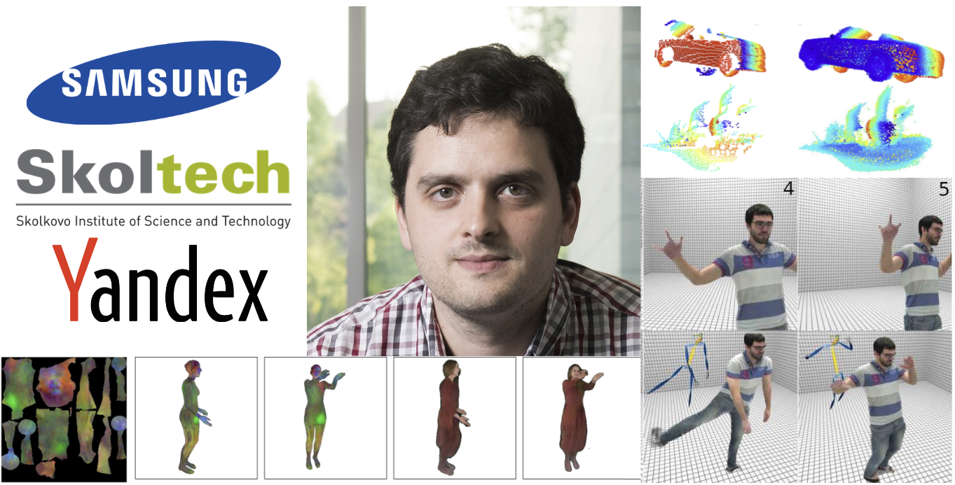
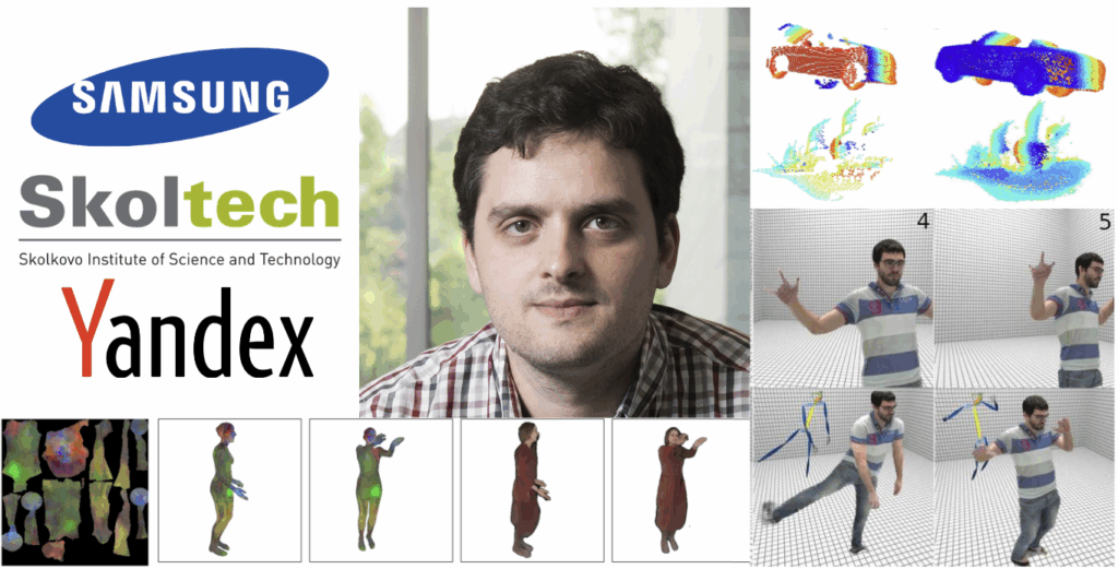
Meet our distinguished guest for the third interview: Professor Victor Lempitsky. Prof. Lempitsky is among the best researchers in machine learning, placing especially highly in the field of computer vision (here is his Google Scholar account). Currently Victor is leading the Computer Vision Group at Skoltech (Skolkovo Institute of Science and Technology) and is the VR project leader at Yandex.

Foreword. Before we begin, I have to say that this interview was composed before February 24, 2022. In fact, it was finalized on February 22, so by now it is almost half a year old. This is the reason why Q6 may look a little strange these days—we were not dancing around the elephant in the room, it simply had not entered yet. By now, Victor has left both positions mentioned in the preamble and is currently working on a new startup in the AR/VR field.

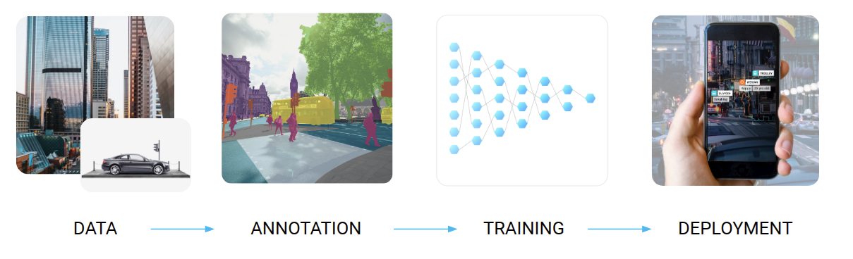
Q1. Hello Victor, and welcome to our interview! Computer vision is your major focus, so let me start off immediately with the obligatory question for our blog: what is your general view on synthetic data for computer vision? Do you agree that synthetic data, understood as artificially generated labeled data used to train machine learning models, can be a feasible way out of the data problem for computer vision? Or do you place more faith in other possible approaches that we’ve previously discussed on this blog: augmentations, mixup and self-adversarial training, few- and zero-shot learning, adding unlabeled data, and others?

I do believe in synthetic data, and several recent projects I was involved with have seen clear benefits from using synthetic data. However, most useful synthetic data are modeled from the real world. Such modeling can benefit strongly from unsupervised learning. So, in the end, there is no dichotomy: I believe in the usefulness of synthetic data, which is enriched/created from real unlabeled data. Augmentations, mixups, adversarial training can all be used as the ways to generate useful synthetic data from real data, even though people not always think about augmentations in this way.

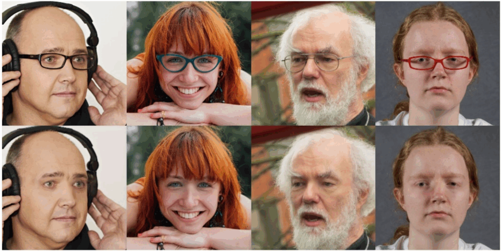
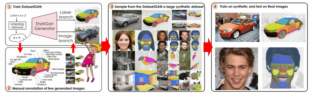
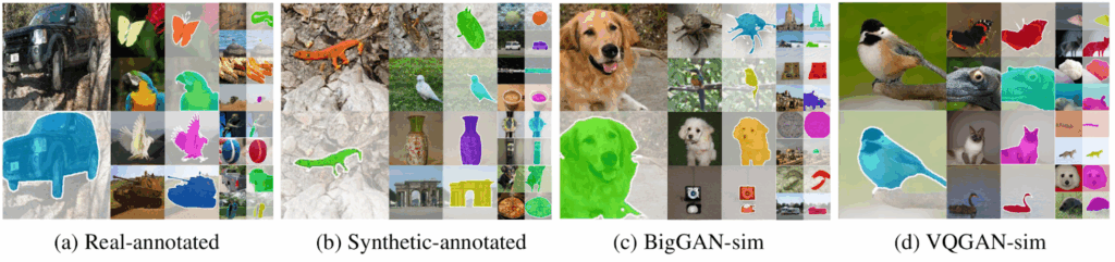
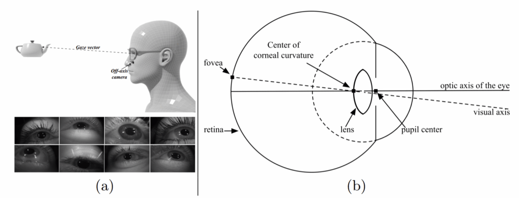
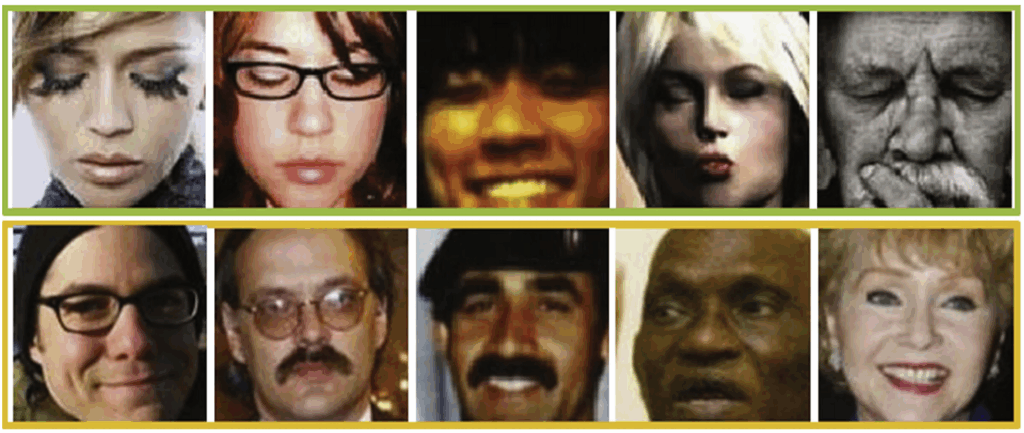
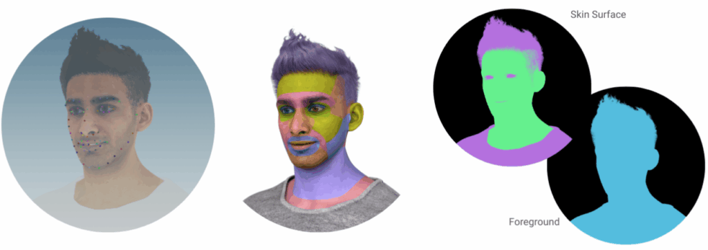
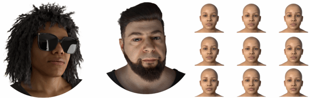
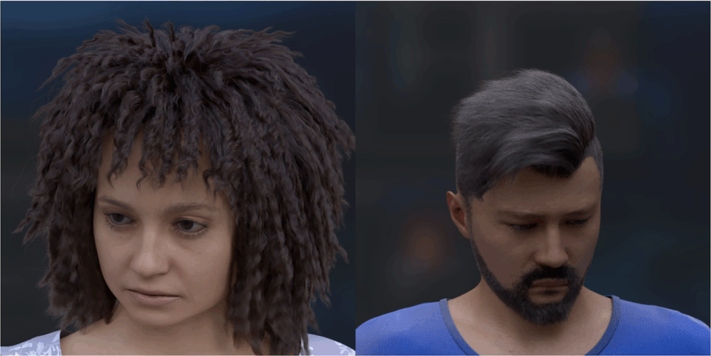
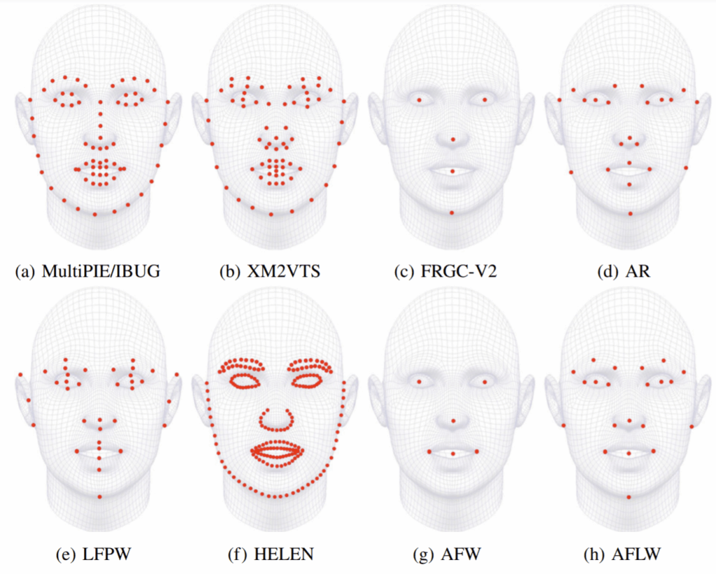
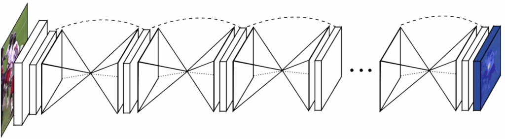
Q2. Much of your most recent work is devoted to image generation. You have created GANs that work without convolutions or self-attention, neural renderers that can dress 3D avatars and generate semi-transparent objects, GANs that generate timelapse videos of landscapes, and much more. In particular, you often work on 3D generation—generating meshes, textures, point clouds—which is the obvious next step after learning to generate flat images. 3D generation is only starting to work well enough for practical applications, but still, the rate of progress in this field is spectacular. I usually show this picture in my lectures on GANs:

Do you expect 3D generation to undergo similarly explosive growth in the near future? Or are there conceptual difficulties that need to be resolved before we get the virtual reality Metaverse generated on the fly with GANs?

The picture you show is indeed very telling, and it reflects and conflates several trends: improvements in algorithms, improvements in computational resources, and improvements in datasets. 

Given how many bright people are now working on 3D data synthesis, I believe that fast progress in algorithms is inevitable. Neural renderers such as PyTorch3D or nvdiffrast are certainly one piece of the puzzle. Computational resources are trickier and a lot of progress will be bottlenecked on them, so I naturally expect that main breakthroughs will come from the “big four” of NVidia, Google/DeepMind, Meta, and Microsoft (all four have brilliant researchers but also huge computational resources). This was to a large degree true even for 2D image generation, and will likely remain even more true for 3D. Note that I am not saying that everybody else should either join those corporations or work on something else. Just like StyleGAN(s) from NVidia created a whole vibrant ecosystem of researchers from different institutes building on top of it, the same will likely happen with 3D.

The main bottleneck for progress in 3D data synthesis, however, is (and will be) datasets. Here things are very different from 2D. With 2D, once algorithms and resources were ready, finding good enough datasets for learning was relatively easy. Note that here I am talking about 2D static image generation, good datasets of HD videos are much harder to get: say, YouTube is largely not HD quality, and it is quite a challenge to scrap video datasets of objects or people in high resolution from YouTube. Getting good and large 3D datasets is much harder, especially if we are talking about “full 3D” and not just 2.5D (i.e. color + depth) or toyish 3D models. Currently, quite a few researchers are trying to bypass this lack of datasets and to learn 3D synthesis by matching the 2D images. To this end, they insert 2D projections into their generation learning pipelines. This is surely interesting and could be fruitful, but is inevitably much harder. Just imagine someone trying to learn StyleGAN-like image synthesis while only having access to a dataset of 1D projections such as row sums or one-pixel slices.

To sum up, I think that the rate of progress in 3D data synthesis will be limited and conditioned on the quality of 3D datasets. Hence, it will be a harder and longer story than with 2D (but no less interesting!)

Q3. Let us continue from the last question, taking generative models yet further into the realm of speculation. I have always viewed image and 3D generation as an inherently finite task. It has not been easy to scale GANs up, but it seems like progress is inevitable. And human eyes have a finite resolution after all (be it 8K, 32K, or 256K), so the models will sooner or later reach this resolution with photorealistic quality, and there will be no point to move any further. 

Do you agree with this view, and if yes, when do you expect image and 3D scene generation to hit this ceiling and provide a perfectly immersive experience? (Let’s limit this question to vision, I understand that full immersion will require other senses as well.)

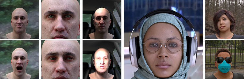
Let me start by noting that the story with 2D image generation is far from over, even if one can generate very realistic human faces. First of all, GANs still have limited diversity and mode coverage (otherwise we will not have dozens of interesting papers on StyleGAN inversion, and very simple approaches would do the job). Diffusion models are better than GANs in covering the whole distribution but are still extremely slow. Furthermore, even though GAN samples for faces are realistic, GAN samples for full body human images or, say, for full body cats are either significantly less realistic or significantly less diverse (or both). Finally, for 2D video synthesis, we as a community are very far from truly realistic results (at least in the unconditional setting).

Regarding 3D, the situation is even harder for the reasons I discussed in the answer to the previous question, so I do not expect perfect photorealism there for quite a few years.

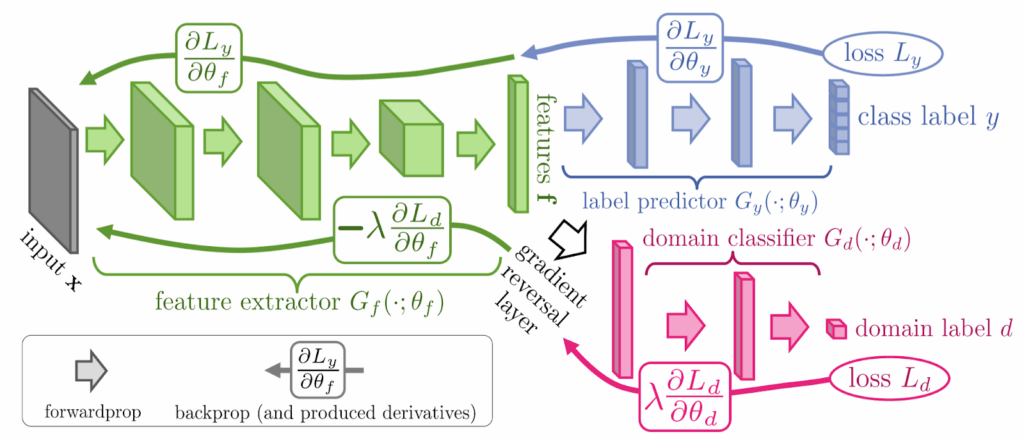
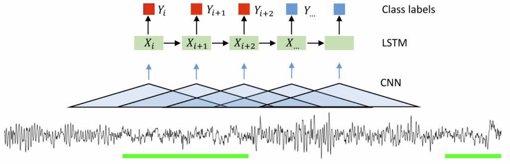
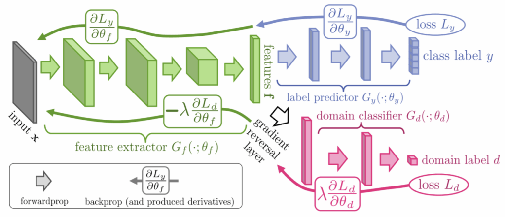
Q4. Now let me ask a (slightly more) technical question that I’ve been interested in for a long time. Your two most cited papers according to Google Scholar are “Unsupervised domain adaptation by backpropagation” (joint work with Yaroslav Ganin) and its continuation and extension, “Domain-adversarial training of neural networks” (with a lot of people including, e.g., Hugo Larochelle). They are also, in my opinion, some of the most relevant for synthetic data because they present a simple and ingenious domain adaptation method.

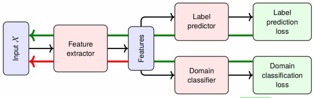
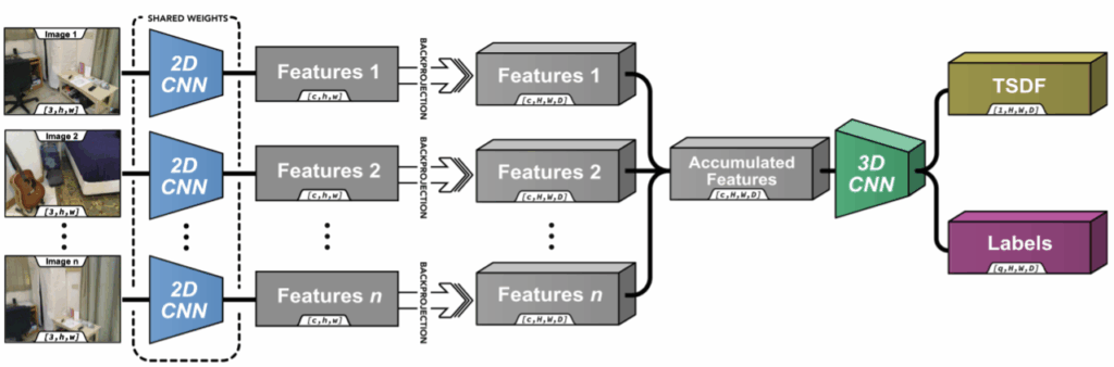
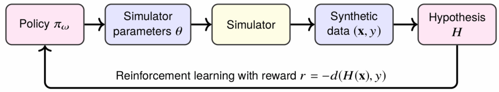
We have just discussed the basic idea of Ganin and Lempitsky (2015) on this blog, so I’ll be very brief in explaining it. The idea goes as follows: suppose you want to have a model that works for both synthetic and real data (or any two domains, really). You want to train a feature extractor that will extract features independently of the domain, so that, say, a synthetic face will have the same features extracted as its real counterpart, and models trained with these features on synthetic data can be applied to real data. To achieve this, you add a domain classifier that predicts whether it was a synthetic or a real image based on the features extracted. You want that classifier to fail, just like you want the discriminator to fail in GANs. So you train it as another head of your network, but the gradients for the classification error function are reversed, optimizing it in the opposite direction. In the illustration below (taken from your papers), the classifier wants to minimize its loss L_d, but by the time it gets to the feature extractor, the loss is inverted, and the extractor is actually maximizing it.

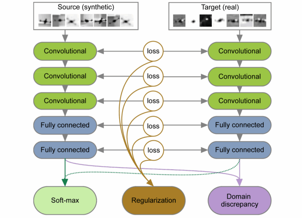
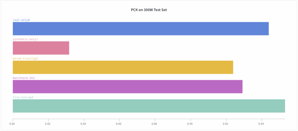
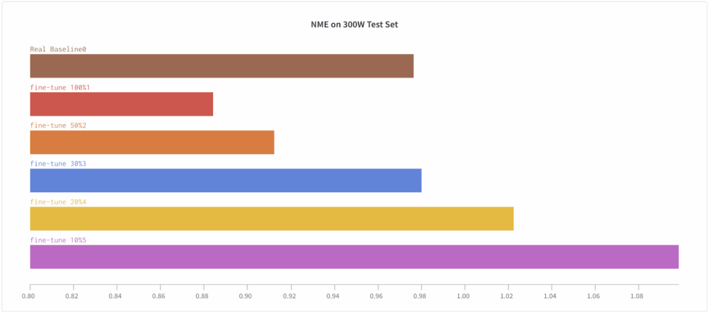
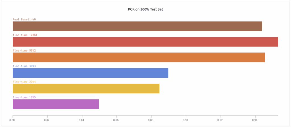
My question here is two-fold. First, I explained your idea in terms of synthetic and real images, and the actual papers also present examples of synthetic-to-real transfer, but only for small images. Have there been attempts to apply this to larger-scale domain adaptation, especially synthetic-to-real, and how successful have they been?

Second, domain-adversarial training sounds like a very general idea that could actually be applicable wider than just domain adaptation. One cannot say this idea is not widely known: both papers have thousands of citations, including foundational works on GANs. But why haven’t GANs switched to gradient reversal instead of alternating training between the generator and discriminator? Are there some hidden problems here that are not evident in the basic idea?

On your first question, indeed the approach has become popular, and there has been a lot of follow-up work including applications to large images. Just as with small images, the approach there works somewhat but without miracles. I.e., it usually beats the no-adaptation baseline quite confidently, but, of course, does not solve the domain gap problem completely. For the second question, indeed almost all GANs separate the steps for the generator and the discriminator updates and do not reuse the gradient. The main reason, I believe, is that most modern GANs use slightly different functionals as objectives for the generator and the discriminator. In particular, it turns out that to get the best GAN performance, it is useful to have some form of the so-called non-saturating objective for the discriminator, and also to regularize the discriminator quite strongly with a proper regularizer (and details of such regularization matter a lot). So, when your generator and discriminator are trying to optimize slightly different functionals, gradient reuse becomes highly non-trivial and is therefore not used. 

Just to clarify, for me the difference between gradient reversal and GANs is not a big deal. Actually, we learned about the GAN arxiv report halfway during the project and by that time we have settled on the idea and the language of “gradient reversal”. This is why we explained our approach in a slightly different way in our paper, and perhaps connected it to GANs in a less clear way than we should have done (but back in early 2015 it was way less obvious that GANs would become such a dominating idea). 

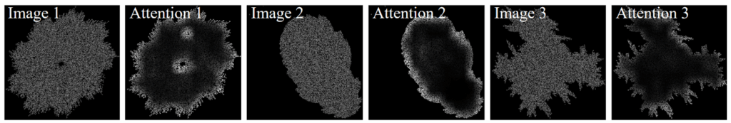
Q5. Another recent work of yours introduces Cloud Transformers, special architectures for processing point clouds that use ideas similar to self-attention blocks, with excellent results in point cloud segmentation, inpainting, and reconstruction tasks.

Since their inception in 2017, Transformers have taken deep learning by storm. They started by basically replacing all other embeddings in natural language processing and serving as the basis for the very best language models, but now they are all over computer vision as well, ever expanding their reach as your own work suggests. It looks a bit like deep learning gradually taking over every field in the early 2010s.

Do you have an explanation for this success? I understand how a Transformer works mathematically, but is there any explanation why self-attention proves to be such a good idea in practice?

Or maybe it’s just an umbrella term for a specific useful trick, and otherwise modern Transformers are very different from each other? In your paper, you keep using words such as “variant” or “reminiscent”, and the architecture indeed doesn’t look much like Vaswani’s original. What is that core idea that makes an architecture a Transformer, and again, why, in your opinion, does it work so well?

Well, it is hard to argue that transformers are the most exciting and impactful thing that has happened in deep learning in recent years. What is most exciting about transformers is their universality. True, we are still witnessing the competition between vision transformer variants and ConvNet architectures for the title of “the king of ImageNet”. But what is remarkable and makes many people excited is that very similar Transformer architectures can solve very different tasks across very different modalities (images, audio, text, action planning, etc) with near state-of-the-art quality. Certainly, it feels like the right thing, as our brains also have remarkable plasticity and can repurpose different parts between modalities.

Our cloud transformers paper will obviously be far less impactful compared to the original transformers, but I still like it very much. Our architecture is similar to “classical” transformers in some ways. E.g. it treats individual points as elements within an unordered set, and our key layer uses multiple processing heads. There are also differences (our equivalent of attention is sparse, and we use convolutions). Still, what I liked about our results is that essentially the same architecture is able to solve very different point cloud processing tasks. This is again reminiscent of the general transformer idea. 

Q6. And finally a (slightly) more personal question. Anyone who knows you personally or at least follows you knows you feel strongly about the ethical use of AI.There is a trend in the computer vision community about ethical usage of CV technologies. For instance, the creator of YOLO object detectors Joseph Redmon quit computer vision in early 2020 and famously explained his decision as follows: “I stopped doing CV research because I saw the impact my work was having. I loved the work but the military applications and privacy concerns eventually became impossible to ignore.”

What is your view on the ethical concerns that arise in modern computer vision? Are researchers responsible for potentially unethical uses of their results? I suppose there is no way to stop progress, but do you think there may be ways to ensure that progress works for the benefit of humanity and not against it? What would you advise to work on if one wanted to achieve this goal?

I had a small project on person re-identification (mostly from surveillance cameras) with my PhD student back in 2016, and after one year or so we stopped. I do not think we pushed state-of-the-art in video surveillance that much, and the reviewers for the submissions we made on the subject concurred with that :). It is the only example where, in retrospect, I sleep slightly better because my work did not make an impact. 

Having said that, some of the good and well-meaning people that I know still work on face recognition and camera-based surveillance, and I do not want to judge them. After all, the camera-based surveillance technology is double-edged. It will most likely benefit strong democratic societies by making life there safer and more convenient, but it will make life in authoritarian and totalitarian societies considerably worse, which we are already starting to witness in Russia and other countries. The same actually goes for AI and automation issues. The net effect will be strongly positive, people will live more meaningful and productive lives with more interesting occupations, but the dystopian scenarios will also materialize in some societies. 

Like always, stopping the progress is impossible, even if many strong researchers including Joe Redmon quit the area. Progress in AI-based surveillance and automation “simply” calls for better and stronger political institutions. And the faster the progress, the more urgent the call. I know this all sounds like I am trying to push the responsibility from AI researchers to others (civil society and politicians), but I am just being honest and realistic. The best thing that we (researchers) can and must do is to inform the general public about the current state-of-the-art and reasonable projections for the future.

Victor, thank you very much for your answers! And you, dear reader, stay tuned for our next interviews!

Sergey Nikolenko
Head of AI, Synthesis AI

Last time, we started a new series of posts: an overview of papers from CVPR 2022 that are related to synthetic data. This year’s CVPR has over 2000 accepted papers, and many of them touch upon our main topic on this blog. In today’s installment, we look at papers that make use of synthetic data to advance a number of different use cases in computer vision, along with a couple of very interesting and novel ideas that extend the applicability of synthetic data in new directions. We will even see some fractals as synthetic data! (image source)

Introduction and the Plan

In the first post of this series, we talked about new synthetic datasets in computer vision. This post is only superficially different from the first one: here we will consider papers that apply synthetic data to various practical use cases, concentrating more on the downstream task than on synthetic data generation. However, the generation part here is also often interesting, and we will definitely discuss it.

I will also take this opportunity to discuss two very interesting developments related to synthetic data. First, we will see that synthetic images do not have to be realistic at all to be helpful for training even state-of-the-art visual Transformers, and it turns out that this has a lot to do with fractals. In the last part, we will see how synthetic data helps to automatically fill in the gaps and provide missing data for few-shot learning. But before that, we will see several use cases where synthetic data has helped solve practical computer vision problems. Among these use cases, today we do not consider papers that help generate synthetic data and papers that deal with generating or modifying virtual humans—these will be the topics for later posts.

Just like last time, I remind you that we have launched OpenSynthetics, a new public database of all things related to synthetic data. In this post, I will again give links to the corresponding OpenSynthetics pages.

Eyeglass removal

In “Portrait Eyeglasses and Shadow Removal by Leveraging 3D Synthetic Data” (OpenSynthetics), Lyu et al. consider an interesting image manipulation problem: removing glasses from a human face. While solving this problem is desirable for applications such as face verification or emotion recognition, eyeglasses are very tricky objects for computer vision: they are mostly transparent but can cast shadows and introduce other complex effects in the image. The model constructed in this work consists of two stages: a cross-domain segmentation network predicts segmentation masks of the glasses and shadows cast by them (this part is trained adversarially in order to extract indistinguishable features from real and synthetic data), and then “de-shadow” and “de-glass” networks remove both:

The whole thing is trained on a mixture of synthetic data and the CelebA dataset (real data), and the authors report much improved results for eyeglass removal:

This system is the main point of the paper, but for me, it was also interesting to read about their synthetic data generation pipeline. Starting from 3D models of eyeglasses and 3D face models, they manually label four nodes where the glasses attach to the face: two fixed nodes on the temples and two floating points on the nose, “floating” meaning that these two points can drift to produce different positions of glasses on the nose. With these four nodes fixed, the system is able to find out the pose for the glasses, combine it with the face, and then the authors proceed to standard rendering in Blender, also generating the masks for glasses and their shadows to train the segmentation model:

And the results are really impressive. Here are some real examples (perhaps cherry-picked, but who cares?..) from the paper:

Crowd counting

The work “Leveraging Self-Supervision for Cross-Domain Crowd Counting” by Liu et al. (OpenSynthetics) deals with a very straightforward application of synthetic data. Crowd counting is a natural use case: it is very hard to label every person on a crowd photo, and using real images raises privacy issues since it is usually impossible to get the consent of everybody in a real-world crowd.

Indeed, there already exists a large synthetic dataset for crowd counting called GCC (Wang et al., 2019) with over 7.6 million people labeled on over 15K synthetic images. This dataset was produced by the Grand Theft Auto V engine, that is, Rockstar Advanced Game Engine (RAGE), together with the Script Hook V library that allows extracting labeling from RAGE. Here are two sample images from the paper, a real crowd on the left and a synthetic one on the right:

Liu et al. use GCC for training and supplement it with unlabeled real images to cope with the domain shift, with a couple of new tricks designed to improve crowd density estimation (such as accounting for perspective since the crowd density appears higher on top of an image such as above than on the bottom). They obtain significantly improved results compared to other domain adaptation approaches; here are a couple of samples (the ground truth crowd density map is in the middle, and the estimated density map is on the right, together with the estimated number of people):

This is an interesting use case for us since it can be read as reaching largely the same conclusions as we did in our recent white paper: if done right, relatively simple combinations of synthetic and real data can work wonders. It is encouraging to see such approaches appear at top venues such as CVPR: I guess synthetic data does just work.

Formula-driven supervised learning for pretraining visual Transformers

And now we proceed from state of the art, but still quite straightforward applications to something much stranger and, in my opinion, more interesting. First, a very unusual application of synthetic data that requires a little bit of context. In 2020, Kataoka et al. presented a completely new approach to training convolutional networks called Formula-Driven Supervised Learning (FDSL). They automatically generate image patterns by assigning image classes with analytically defined fractal categories. It raises a separate and quite difficult problem of how to do that, but the important thing is that after this transformation, you get a family of fractals for each image category. Here is an illustration from Kataoka et al.:

As you can see, synthetic fractal images are far from realistic, but they capture some of the patterns characteristic for a given class and hence can be used to pretrain deep learning models; as usual with synthetic data, one can generate an endless stream of new samples from these fractal families. This pretraining does not make training on real images unnecessary but can improve the final results.

Well, in 2022 Kataoka et al. made the next step (OpenSynthetics), moving from CNNs to visual Transformers. They developed new techniques for their synthetic generation, including a new dataset of families focused on image contours. It turned out that visual Transformers pay most attention to the contours anyway, so even a textureless image is helpful for pretraining:

And visual Transformers perform better when they are pretrained on images like this one instead of real photos! For example, the authors report that ViT-Base pre-trained on ImageNet-21k showed 81.8% top-1 accuracy after fine-tuning on ImageNet-1k, while the same model with FDSL shows 82.7% top-1 accuracy when pre-trained under the same conditions.

In my opinion, this is a very interesting direction of study. Apart from its direct achievements, it also shows that synthetic-to-real domain shift is not necessarily a bad thing, and if the data is generated in the right way, trying to achieve photorealism may not be the right way to go.

Synthetic Representative Samples for Few-Shot Learning

This last paper for today is a little bit of a stretch to call synthetic data, but it’s another interesting idea that may have applications for synthetic data generation as well. Last time, we discussed BigDatasetGAN, a generative model able to create images already labeled for semantic segmentation. This may be one of the first steps towards solving the problem of synthetic data: until the works on DatasetGANs, nobody could generate labeled data so nobody could use generative models to directly generate useful synthetic images.

If we are talking about classification rather than segmentation, it looks much easier to sidestep this issue: ever since BigGAN, generative models could produce realistic-looking images in many different categories. But this raises another question: to train a generative model we need a dataset in this category, so why don’t we just take this dataset to train on instead of generating new samples?

The work “Generating Representative Samples for Few-Shot Classification” (OpenSynthetics) by Xu and Le, a collaboration between Stony Brook University and Amazon, finds a new use case where this kind of conditional generation can be useful. The basic idea is as follows: in few-shot learning, say for image classification, one usually trains a feature extractor on a dataset with plenty of labeled data (but the wrong classes) and then adapts it to new classes by estimating a prototype sample. Then this sample can be used for classification; here is an illustration for few-show and zero-shot classification via prototypes from a classical paper by Snell et al. that started this field:

This illustration works in the latent space of features produced by some kind of encoder.

But this prototype-based idea has a drawback: it is hard to find a representative prototype if all you have are a few samples. Even if you have a perfect encoder that produces smooth and wonderfully separated Gaussians for every class, these Gaussians have a core of central representative samples and also non-representative samples that are further from the center:

And if we base a classifier on a single prototype that turns out to be non-representative, the results can be far from perfect. Here is an illustration from an ICLR 2021 paper by Yang et al.:

But how do we achieve this kind of calibration? Xu and Le propose—and this is where the relation to synthetic data comes into play—to generate representative samples from a variational autoencoder. It is common to use conditional VAEs to learn to extract representative features from images, but this time the cVAE is restricted to produce only representative, central examples of a class (feature vectors close to the center of a Gaussian) via sample selection:

Note the semantic embedding a: this is where the new samples will come from. For a new class, the authors take its semantic embedding, plug it into this VAE’s decoder, and generate representative samples for the new class. Then the resulting generated prototype is either mixed with actual samples (in few-shot classification) or not (in zero-shot classification), with improved results on miniImageNet and tieredImageNet.

This is definitely a non-representative example of a paper on synthetic data: the “data” is actually in feature space, and the problem is image classification rather than anything with complicated labeling. But this direction, dating back at least to 2018 (Verma et al., CVPR 2018), is an interesting tangent to our space, and just like DatasetGAN, it goes to show a way in which generative models may prove useful for synthetic data generation.

Conclusion

In this post, the second in the CVPR ‘22 series, we have discussed several use cases of synthetic data that have been advanced at the conference, starting from straightforward applications such as eyeglass removal and crowd counting and progressing to less obvious ideas of how deep generative models and even regular mathematical models such as fractals can help produce synthetic data useful for machine learning. Next time, we will discuss a more specific use case related to synthetic humans; stay tuned!

Sergey Nikolenko
Head of AI, Synthesis AI

CVPR 2022, the largest and most prestigious conference in computer vision and one of the most important ML venues in general, has just finished in New Orleans. With over 2000 accepted papers, reviewing the contributions of this year’s CVPR appears to be a truly gargantuan task. Over the next series of blog posts, we will attempt to go over the most interesting papers directly related to our main topic: synthetic data. Today, I present the first but definitely not the last installment devoted to papers from CVPR 2022.

New Synthetic Datasets: Beyond Images

As always, CVPR is large, and it contains multitudes, but this year one of the main topics is neural radiance fields (NeRF). These models seem to be the new GANs today, or, better to say, new visual Transformers that were in turn the new GANs a couple of years ago. We view image synthesis, especially controlled synthesis with 3D information, as a key idea that can propel synthetic data forward, so I plan to devote several upcoming posts to recent NeRF advancements.

But in this series, let me begin with more straightforward applications of synthetic data that have found their way into the CVPR program this year. On the list today we have several new synthetic datasets, usually related to specific use cases of synthetic data; many of them touch upon problems that we have already discussed on this blog but some introduce entirely new avenues for research.

Synthetic data is a well-established field, and this blog has already documented many of its achievements. By now, it is not enough to just generate a new synthetic dataset to get to a top conference like CVPR (to be honest, it was never enough): you need some twist on the tried-and-true formula of “make or obtain 3D CG models, render images, train CV models, profit”. In this section, let us see what new twists CVPR 2022 has brought.

And one more thing before we begin: we have recently made public a new database that will gradually collect all things related to synthetic data. It is called OpenSynthetics, and it already has quite a lot of content on synthetic datasets, papers, and code repositories related to synthetic data. So in these review posts, I will also give links to the corresponding OpenSynthetics pages.

BigDatasetGAN: Generating ImageNet1K with Labels

It had always been common wisdom that GANs, despite their excellent image generation quality and usefulness for synthetic-to-real refinement, cannot really help with data generation from scratch: there was no way to generate labeled data and no easy way to label generated images. Basically, ever since ProGAN and BigGAN (OpenSynthetics; both released in 2018) you could use GANs to generate new realistic images with sufficient quality, but you would still have to label them afterward as if they were just new images. And this has always meant that GANs are useless for synthetic data generation: we have never lacked new images of ImageNet categories, the bottleneck has always been in the labeling.

Well, it looks like there is a way to generate labeled data now! This research direction, driven by NVIDIA researchers, bore its first fruit last year when Zhang et al. presented DatasetGAN on CVPR 2021. Their pipeline works as follows: use StyleGAN to generate several images (say, cars), hand-annotate a few of them for your task (say, segmentation of various car parts), and train a very small model (style interpreter) to produce similar segmentation masks from StyleGAN features. At the cost of labeling a few images (literally, a few: DatasetGAN required 16 labeled heads or about 1000 polygons), you can use StyleGAN to generate as many labeled images as you wish, with the usual excellent StyleGAN quality:

On this year’s CVPR, Li et al. continued this line of research and introduced BigDatasetGAN based on BigGAN instead of StyleGAN. The difference is that BigGAN is better suited for generating a wide variety of different image categories, so now you can hand-label 8000 images, 8 for each category, and have a single model able to produce 1000 ImageNet1K categories that come pre-labeled for segmentation:

The authors report results improved over supervised pretraining for standard segmentation models.

Does this mean that synthetic data is soon to be absorbed into deep generative models? Time will tell, but I am not sure: generative models are still hard to train, and this approach requires an operational large-scale GAN with the desired categories before we go into labeling. Moreover, DatasetGANs deal only with segmentation so far, and I have my reservations about more complex labeling such as depth. Still, this is an exciting development that shows the power of modern generative models, and its results provide a set of completely new tools for the arsenal of synthetic data generation.

ABO: Real-World 3D Object Understanding

ABO stands for Amazon Berkeley Objects (OpenSynthetics), a new indoor environment and object dataset presented in the work by Collins et al., who are, you guessed it, researchers from UC Berkeley and Amazon. ABO answers the same need as the classical but sadly unavailable SunCG dataset, ShapeNet, or Facebook AI Habitat: it provides a large-scale catalogue of 3D models of indoor household objects—chairs, shoes, coat hangers, rugs, tables, and so on—that can be placed in a variety of indoor environments with available renderings.

Since Amazon is… well, Amazon, ABO is based on product listings: the dataset contains nearly 150K listings of 576 product types with hi-res photos and over 8000 turntable “360° view” images. It also includes nearly 8000 handmade high-quality 3D models of various objects. Moreover, and this is unique to ABO, the objects come with attributes that identify their material, which is useful for physically-based rendering:

The authors show that training on ABO leads to better results than training on ShapeNet for state-of-the-art 3D reconstruction models. They also introduce a new task that has been enabled by their work, material estimation, and present novel network architectures for this task. In general, this is an impressive effort, and I hope that it will enable many new works in 3D scene understanding, indoor navigation, and related fields:

ObjectFolder 2.0: A Multisensory Object Dataset

While ABO provides some information about the material of the object, it is far from exhaustive. Stanford researchers Gao et al. attempt a far more ambitious task in their new ObjectFolder 2.0 dataset (OpenSynthetics): they aim to model complete multisensory profiles of real objects. This means that they aim to capture not only the 3D shape and material of an object (and therefore its texture) but also other sensory modalities including audio (how a cup clinks when you touch it with a spoon) and feeling to the touch. This information can be later used for problems such as contact localization (where exactly have I touched this object?) that are both difficult and important in robotics:

Since all of these modalities are location-dependent, they cannot all be explicitly stored in the dataset. The authors use implicit neural representations, that is, each object is defined by a few neural networks (multilayer perceptrons) that are trained to convert coordinates into whatever is necessary; VisionNet models the neural scattering function, AudioNet models the location-specific part of the audio response from applying a unit force to this location, while TouchNet predicts the deformation map and tactile image (geometry of the contact surface):

ObjectFolder 2.0 contains these representations for 1000 household objects such as cups, chairs, pans, vases, and so on.

Gao et al. test their dataset with three downstream tasks that require multimodal sim2real object transfer: object scale estimation based on vision and audio, contact localization based on audio and tactile response, and shape reconstruction based on visual and tactile data. They report improved performance across all tasks, and this dataset indeed looks like a possible next step for object manipulation in robotics.

Articulated 3D Hand-Object Pose Estimation

Pose estimation is a classical computer vision problem; as in all problems related to the understanding of the 3D world from 2D images, synthetic data comes to mind naturally: it is impossible to do exact manual labeling for pose estimation, and even inexact human labeling is very copious. This goes double for more detailed tasks such as hand pose estimation, so it is no wonder that there exist synthetic datasets for this problem; in particular, here at Synthesis AI we have a variety of hand gestures as part of our HumanAPI.

In “ArtiBoost: Boosting Articulated 3D Hand-Object Pose Estimation via Online Exploration and Synthesis” (OpenSynthetics), Li et al. make the next step: they consider not just hand gestures but hands holding various objects in different positions. The authors consider the “composited hand-object configuration and viewpoint space” (CCV space) where you can vary object types, composite hand-object poses, and camera viewpoints:

Then they apply a newly developed grasp synthesis method (that I will not go into), obtain renderings of a synthetic hand grasping the object, and use these images for training.

What is most interesting for me in this work is that it is an example of the “closing the loop” idea that we have been proposing for quite some time ago here at Synthesis AI; in particular, pardon the self-promotion, I discussed it as an important idea for the future of synthetic data in Chapter 12 of my book.

In this case, Li et al. do not merely sample the CCV space and create a randomly generated dataset of synthetic hands with objects. They assign weights to different objects, poses, and viewpoints, and update these weights with feedback obtained from the trained model, trying to skew the sampling towards hard examples, a technique known in other contexts as “hard negative mining”. It is great to see that “closing the loop” is gaining traction, and I am certain it can help in other problems as well.

SHIFT: Synthetic Driving via Multi-Task Domain Adaptation

And now let us, pardon the pun, shift to data about the outdoors. We begin with autonomous driving. The work “SHIFT: A Synthetic Driving Dataset for Continuous Multi-Task Domain Adaptation” (OpenSynthetics), coming from ETH Zurich researchers Sun et al., is a pure synthetic dataset presentation for SHIFT, a synthetic driving dataset—but SHIFT is far from a “regular” synthetic dataset with some labeled images! The problem that Sun et al. recognize here is that autonomous driving requires the system to adapt to constantly changing conditions: if you are driving and it starts raining, the view around you changes significantly and maybe quite quickly, and the computer vision system has to keep working fine.

To help cope with that, SHIFT contains explicit “domain shifts” across several different domains such as weather conditions, time of day, surroundings, and so on:

So far this is quite standard fare for autonomous driving simulators. What’s more, SHIFT provides continuous shifts across domains whenever possible. You can have day gradually turning into night or rain starting on a sunny day:

Naturally, each frame is annotated in the usual modalities, with object bounding boxes, segmentation maps, depth maps, optical flow, and LiDAR point clouds.

Based on SHIFT, the authors investigate how various object detection and segmentation models cope with these domain shifts. They demonstrate that conclusions about robustness to domain shift that can be made on synthetic data also transfer to real datasets. I think that’s an important validation for synthetic data in general: it turns out that synthetic data can help evaluate machine learning models in ways that real data may fail to provide.

TOPO-DataGen: Multimodal Synthetic Data Generation for Aerial Scenes

In another classical synthetic data paper, EPFL researchers Yan et al. present TOPO-DataGen (OpenSynthetics), an automated synthetic data generation system that utilizes available geographic data such as LiDAR point clouds, orthophotographs, or digital terrain models to create synthetic scenes of various parts of the world, complete with the usual synthetic modalities such as depth maps, normals, segmentation maps, and so on:

Generated images look very impressive and highly realistic, which is made slightly easier by the fact that they are aerial images taken from far away. Based on TOPO-DataGen, Yan et al. develop a new CrossLoc model for absolute localization (i.e., estimating the 6D camera pose in space) that works with several input modalities. They also show some impressive demos of trajectory reconstruction from aerial images based on CrossLoc. In general, while synthetic satellite and aerial images have already been generated, I believe this is the first attempt to bring together the different modalities that are actually often available in current practice.

LiDAR snowfall simulation

Finally, a very specific but fun use case: simulating snowfall. Autonomous driving should work under all realistic weather conditions, including heavy snow. But snow presents two problems that are especially bad for LiDARs: first, the ground becomes wet, which changes its reflective properties, and second, the particles of snow in the air also interact with the laser beam, leading to absorption and backscattering that attenuate and introduce a lot of noise into the LiDAR signal.

Hahner et al. present a snowfall simulation system able to augment synthetic LiDAR datasets (in this case, STF by Bijelic et al. that itself introduced a fog simulation system) with special models for wet ground reflection and the influence of scattering particles. As a result, 3D object detection models trained with this augmentation perform much better; in the illustration below, note that the rightmost results contain no spurious objects, and predicted bounding boxes (black) match the ground truth (green) very well:

Conclusion

Today, we have begun our long journey through CVPR 2022. We have looked at papers that introduce new synthetic datasets, usually going far beyond simple generation of labeled images and sometimes defining completely new tasks. Next time, we will talk about papers that present specific use cases for synthetic data, that is, validate the use of synthetic data in practical computer vision tasks. Admittedly, it’s a blurry line with this first installment, but this post is getting quite long as it is. Until next time, stay tuned to the Synthesis AI blog, and check out OpenSynthetics!

Sergey Nikolenko
Head of AI, Synthesis AI

After a long hiatus, we return from interviews to long forms, continuing (and hopefully finishing) our series on how synthetic data is used in machine learning and how machine learning models can adapt to using synthetic data. This is our seventh installment in the series (part 1, part 2, part 3, part 4, part 5, part 6), but, as usual, this post is (I hope!) sufficiently self-contained. We will discuss how one can have a model that works well on synthetic data without making it more realistic explicitly but doing the domain adaptation work at the level of features or model itself.

Intro and weight sharing

In previous installments, we have considered models that perform refinement, that is, domain adaptation at the data level. This means that somewhere in the model, there is a learned transformation that takes data points from the source domain (in our case, synthetic images) and transforms them to make them more like the target domain (real images). 

But it sounds like a lot of unnecessary extra work! Our final goal is very rarely to generate more realistic synthetic images. On the contrary, we want to use synthetic images to help train better models; the data itself is not important, it is just a stepping stone to models that work better. So maybe we don’t need to learn transformations on the level of images and can work in the space of features or model weights, never going back to change the actual data?

One simple and direct approach to doing that would be to share the weights among networks operating on different domains. This way, when you train on both domains, the network has to learn to do well on both with the same weights – exactly what you need for domain adaptation. This was the idea of the earliest approaches to domain adaptation in deep learning, but weight sharing and similar ideas remain relevant to this day. For instance, Rozantsev et al. (2019) do domain adaptation with a two-stream architecture; the weights for processing the two domains are not shared but the architectures are the same, and there are special regularizers on all layers that bring their weights together:

Another approach to model-level domain adaptation is to mine relatively strong priors from real data that can then inform a model trained on synthetic data, helping fix problematic cases or incongruencies between synthetic and real data. This also brings us to curriculum learning: it is often helpful to start with the easy cases and get a network rolling, and then fine-tune it in harder and harder situations.

For example, Zhang et al. (2017) present a curriculum learning approach to domain adaptation for semantic segmentation of urban scenes. They train a segmentation network on synthetic data (specifically on the GTA dataset) but with a special component in the loss function related to the general label distribution in real images, intended to bring together the distributions of labels in real and synthetic datasets. The problem here is that this distribution is not available in real data, so this is where curriculum learning comes in: the authors first train a simpler model on synthetic data to estimate the label distribution from image features and then use it to inform the segmentation model:

But there are much more interesting ideas in model-based domain adaptation than just training the same network on both domains with some regularizers. Let’s get to them!

Reversing the Gradients

One of the main directions in model-level domain adaptation was initiated by Ganin and Lempitsky (2015) who presented a generic framework for unsupervised domain adaptation. Their basic approach goes as follows:

Let’s unpack what we see in this picture:

• the feature extractor, true to its name, extracts features from input data; this is actually the network that we want to make domain-independent; after extraction, the features go two separate ways;
• the label predictor actually does what the network is supposed to do, in this case probably classification but it could be segmentation or any other kind of computer vision problem;
• the domain classifier is the core of this idea; it takes extracted features as input and attempts to classify which domain the original input belonged to.

The idea is to train the label predictor to perform as well as possible and at the same time make the domain classifier perform as badly as possible. This is actually very similar to GANs (which we have discussed before). The difference, however, is that Ganin and Lempitsky devised an ingenious method for training that doesn’t require solving any minimax problems or iteratively alternating between networks. 

The method is called gradient reversal: multiplying the gradients by a negative constant as they pass from the domain classifier to the feature extractor. In this way, the domain classifier learns to maximize its error, and the label predictor minimizes it, all at the same time and within the same loss function. Like this:

In a subsequent work, Ganin et al. (2016) generalized this domain adaptation approach to arbitrary architectures and experimented with domain adaptation in different domains, including image classification, person re-identification, and sentiment analysis. 

Disentanglement: Domain Separation Networks and beyond

Domain separation networks by Bousmalis et al. (2016) represent a different take on the same problem. They attempt to solve domain adaptation via disentanglement, a very important notion in deep learning. Disentanglement is the process of separating different features extracted by a machine learning model so that these separate parts would have different recognizable meanings. For example, many style transfer models (we discussed it in Part IV of this series) try to explicitly disentangle style from content, and then swap the style part of the features before decoding back in order to get the same image in a different style.

In domain adaptation, disentanglement amounts to separating domain-specific features from domain-independent ones, and trying to make sure that the latter will suffice to solve the actual problem. Domain separation networks explicitly separate the shared and private components of both source and target domains, extracting them with a shared encoder and two private encoders, one for the source domain and one for the target domain:

The overall objective function for a domain separation network consists of four parts (let’s not do the formulas, it is, after all, almost Christmas):

• supervised task loss in the source domain, e.g., classification loss;
• reconstruction loss that compares original samples (both real and synthetic) and the results of a shared decoder that tries to reconstruct the images from a combination of shared and private representations;
• difference loss that encourages the hidden shared representations of instances from the source and target domains to be orthogonal to their corresponding private representations;
• similarity loss that encourages the hidden shared representations from the source and target domains to be similar to each other; again, “similar” here means that they should be indistinguishable by a domain classifier trained through the gradient reversal layer, as above.

Bousmalis et al. evaluate their model on several synthetic-to-real scenarios, e.g., on synthetic traffic signs and synthetic objects from the LineMod dataset.

Domain separation networks became one of the first major examples in domain adaptation with disentanglement, where the hidden representations are domain-invariant and some of the features can be changed to transition from one domain to another. Further developments include:

• FCNs in the Wild by Hoffman et al., where feature-based DA for semantic segmentation is done with fully convolutional networks (FCN) where ground truth is available for the source domain (synthetic data) but unavailable for the target domain (real data); they also used domain adversarial training;
• Xu et al. (2019) used adversarial domain adaptation to transfer object detection models—single-shot multi-box detector (SSD) and multi-scale deep CNN (MSCNN)—from synthetic samples to real videos in the smoke detection problem;
• Chen et al. (2017) construct the Cross City Adaptation model that brings together features from different domains, with semantic segmentation of outdoor scenes in mind; they adapt segmentation across different cities around the globe and show that their joint training approach with domain adaptation improves the results significantly;
• and many more…

The last paper I want to highlight here is by Hong et al. (2018) who provide one of the most direct and most promising applications of feature-level synthetic-to-real domain adaptation. In their Structural Adaptation Network, the conditional generator takes as input the features from a low-level layer of the feature extractor (i.e., features with fine-grained details) and random noise and produces transformed feature maps that should be similar to feature maps extracted from real images:

To achieve this, the conditional generator produces a noise map and then adds it to high-level features. Hong et al. compared the Structural Adaptation Network with other state of the art approaches, including FCNs in the Wild and Cross-City Adaptation, with source domain datasets SYNTHIA and GTA and target domain dataset Cityscapes; they conclude that this adaptation significantly improves the results for semantic segmentation of urban scenes. Here is a sample of their results:

Conclusion

Feature-level domain adaptation provides interesting opportunities for synthetic-to-real adaptation. Many of these methods still mostly represent work in progress, but the field is maturing rapidly, and in our experience, feature- and model-level DA is usually a simpler and more robust approach, easier to get to work, so we expect new exciting developments in this direction and recommend to try this family of methods for synthetic-to-real DA (unless actual refined images are required).

With this, I am concluding this long series on different facets of using synthetic data in machine learning. Most importantly, synthetic data is a source of virtually limitless perfectly labeled data. It has been explored in many problems, but we believe that many more potential use cases still remain. Maybe we will get a chance to explore them together in 2022.

Sergey Nikolenko
Head of AI, Synthesis AI

Today, we are talking about the Metaverse, a bold vision for the next iteration of the Internet consisting of interconnected virtual spaces. The Metaverse is a buzzword that had sounded entirely fantastical for a very long time. But lately, it looks like technology is catching up, and we may live to see the Metaverse in the near future. In this post, we discuss how modern artificial intelligence, especially computer vision, is enabling the Metaverse, and how synthetic data is enabling the relevant parts of computer vision.

What is the Metaverse

The Metaverse is far from a new idea. Anyone familiar with the cyberpunk genre will immediately recognize the concept of a virtual reality that characters of William Gibson’s Neuromancer (1984) inhabit. The term itself was coined in Neal Stephenson’s novel Snow Crash (1992), and this virtual reality-based Internet 2.0 has seen many fictionalized adaptations ever since, including The Matrix, Ready Player One, a recent Amazon series Upload, and many more.

While the Metaverse has long been the subject of sci-fi, by now many visionaries believe that developments in VR, AR, and related fields may soon enable similar experiences in real life… I mean, in virtual life, but real virtual life… you know what I mean. One of the sources that got me thinking about the Metaverse recently was a long interview with Mark Zuckerberg. He talks about “the successor to the mobile internet… an embodied internet, where instead of just viewing content — you are in it… present with other people as if you were in other places”. It sounds like Facebook believes in the VR and AR technology and sees the clunkiness of current generation devices as the main obstacle: right now hardly anybody would want to do their jobs in a VR helmet. As soon as wearable technology becomes miniature and light enough, the Metaverse will be upon us.

Mark Zuckerberg motivates this vision, in particular, with mobile workstations: “…you can walk into a Starbucks… and kind of wave your hands and you can have basically as many monitors as you want, all set up, whatever size you want them to be… and you can just bring that with you wherever you want.” Facebook calls this idea the “infinite office.” But in my opinion, it is almost inevitable that entertainment will be the main driving force behind the Metaverse: imagine that you don’t need large screens to have an immersive cinematic experience, imagine your friends on social networks (well, maybe one social network in particular) streaming their experiences through AR glasses, imagine immersive 3D games that enable real human-to-human personal interaction… Well, I’m sure you’ve heard pitches for the VR technology many times, but this time it sounds like it really has a chance of coming through and becoming the next big thing. Others are beginning to build their own vision for the Metaverse including Epic Games, Roblox, Unity, and more. 

How the Metaverse is enabled by computer vision

But we need more than just smaller VR helmets and AR glasses to build the Metaverse. This hardware has to be supported by software that makes the transition between the real and virtual worlds seamless—and this would be impossible without state of the art computer vision. Let me make just a few examples.

First, the obvious: VR helmets and controllers need to be positioned in space very accurately, and this tracking is usually done with visual information from cameras, either installed separately in base stations or embedded into the helmet itself. This is a basic computer vision problem of simultaneous localization and mapping problem (SLAM). VR helmet technology has recently undergone an important shift: earlier models tended to require base stations (“outside-in” tracking), and latest helmets can localize controllers accurately with embedded cameras (“inside-out” tracking) so you don’t need any special setup in the room (image source):

This is a result of progress in computer vision, the cameras themselves have not improved that much.

This problem becomes harder if we are talking about augmented reality: AR software also needs to understand its position in the world, but it needs a far more detailed and accurate 3D map of the environment in order to be able to augment it for the user. Check out our latest AI interview with Andrew Rabinovich, who was the Director of Deep Learning at Magic Leap, the startup that tried to do exactly this.

Second, we have already talked many times about gaze estimation, i.e., finding out where a person is looking by the picture of their face and eyes. This is also a crucial problem for AR and VR. In particular, current VR relies upon foveated rendering, a technique where the image in the center of our field of view is rendered in high resolution and high detail, and it becomes progressively worse on the periphery; for an overview see, e.g., Patney et al. (2016). This is, by the way, exactly how we ourselves see things; we see only a very small portion of the field of view clearly and in full detail, and peripheral vision is increasingly blurry (illustration by Rooney et al., 2017):

Foveated rendering is important for VR because VR has an order of magnitude larger field of view than flat screens, and requires a high resolution to support the illusion of immersive virtual reality, so rendering it all in this resolution would be far beyond consumer hardware.

Third, when you enter virtual reality, you need an avatar to represent you; current VR applications usually provide stock avatars or forgo them entirely (many VR games represent the player as just a head and a pair of hands), but an immersive virtual social experience would need photorealistic virtual avatars that represent real people and can capture their poses, . Constructing such an avatar is a very hard computer vision problem, but people are making good progress on it. For instance, a recent work by Victor Lempitsky’s team introduced textured full-body avatars able to capture poses in real time by visual data streaming from several cameras:

We are still not quite there, especially when it comes to faces and emotions, but we are getting better, and the Metaverse will definitely make use of this technology.

These are only a few of the computer vision problems that arise along the way to the Metaverse; for a more, pardon the pun, immersive experience just look at the list of talks on the recent IEEE VR Conference, where you will see all of these topics and much more.

Synthetic data and the Metaverse

Our long-time readers have no doubt already recognized where this blog post is going. Indeed, as we have discussed many times before (e.g., here or here), modern computer vision is requiring increasingly large datasets, and manual labeling simply stops working at some point. At Synthesis AI, we are proposing a solution to this problem in the form of synthetic data: artificially generated images and/or 3D scenes that can be used to train machine learning models.

I chose the three examples above because they each illustrate different uses of synthetic data in machine learning. Let us go over them again.

First, SLAM is an example where synthetic data can be used in a straightforward way: construct a 3D scene and use it to render training set images with pixel-perfect labels of any kind you would like, including segmentation, depth maps, and more. We have talked about simulated environments on this blog before, and SLAM is a practical problem where segmentation and depth estimation arise as important parts. Modern synthetic datasets provide a wide range of cameras and modalities; for example, here is an overview of a recently released dataset intended specifically for SLAM (Wang et al. 2020):

Second, gaze estimation is an interesting problem where real data may be hard to come by, and synthetic data comes to the rescue. I have already used gaze estimation on this blog as a go-to example for domain adaptation, i.e., the process of modifying the training data and/or machine learning models so that the model can work on data from a different domain. Gaze estimation works with relatively small input images, so this was an early success for GANs for synthetic-to-real refinement, where synthetic images were made more realistic with specially trained generative models. Recent developments include a large real dataset, MagicEyes, that was created specifically for augmented reality applications (Wu et al., 2020); in fact, it was released by Magic Leap, and we discussed it with Andrew last time:

Third, virtual avatars touch upon synthetic data from the opposite direction: now the question is about using machine learning to generate synthetic data. We talked about capturing the pose and/or emotions from a real human model, but there is actually a rising trend in machine learning models that are able to create realistic avatars from scratch. Instagram is experiencing a new phenomenon: virtual influencers, accounts that have a personality but do not have a human actually realizing this personality. Here is Lil Miquela, one of the most popular virtual influencers:

From a research perspective,, this requires state of the art generative models that are supplemented with synthetic data in the classical sense: you need to create a highly realistic 3D environment, place a high-quality human model inside, and then use a generative model (usually a style transfer model) to make the resulting image even more realistic. In this direction, it is still a long way to go before we can have fully photorealistic 3D avatars ready for the Metaverse, but the field is developing very rapidly, and this long way may be traversed in much less time than we have ever expected.

The Metaverse is an ambitious vision straight out of science fiction, but it looks like the Metaverse is becoming increasingly realistic. It is quite possible that you and I will live to see an actual Metaverse, be it a social-centric Facebook 2.0 envisioned by Mark Zuckerberg, massively multiplayer OASIS out of Ready Player One, or, God forbid, the all-encompassing Matrix. But before we get there, there are still many research problems to be solved. Most of them lie in the field of computer vision, and this is exactly where synthetic data is especially effective for machine learning. Join us next time for another installment on synthetic data!

Sergey Nikolenko
Head of AI, Synthesis AI

Today, I am proud to present our guest for the second interview, Dr. Andrew Rabinovich. Currently, Andrew is the CTO and co-founder of Headroom Inc., a startup devoted to producing AI-based solutions for online business meetings (taking notes, detecting and attracting attention, summarization, and so on). Dr. Rabinovich has produced many important advances in the field of computer vision (here is his Google Scholar account), but he is probably best known for his work as the Director of Deep Learning at Magic Leap, an augmented reality startup that raised more than $3B in investments.

Q1. Hello Andrew, and welcome! Let me begin with a general question that I will also expand upon later. You have a lot of experience in academia, with numerous papers published at top conferences and receiving hundreds of citations. At the same time, some of your top accomplishments are related to more “industrial” research work at startups such as Magic Leap.

What kind of work has been more fulfilling for you? And what, in your view, are the main differences in the process and/or results? On the surface, research work in both industry and academia is supposed to produce novel solutions that work well for the problem at hand; are there important differences here?

Hello Sergey, I am glad to be here and thank you for the invitation. What you guys, at Synthesis, are doing is extremely important for the computer vision field, and I am grateful that with these efforts the state of the art in Computer Vision, and AI in general, will improve for many years to come. 

This is a very interesting question that dates back to my undergraduate days when I worked on medical image analysis and was interested in building image cytometers — automated microscopes with machine learning inference skills. While developing the cytometer, it quickly became apparent that the state of the art in computer vision (it was called image processing then) wasn’t quite up to par to solve the practical problems I was facing. This realization made me turn to more theoretical work and focus on developing core vision algorithms. A similar situation happened at Google, where I was really excited to work on algorithms for Google Goggles, the first AR app for Android and iPhone. Then existing, pre-deep learning approaches, weren’t satisfactory to develop product features we were interested in. Again, I turned to more academic research and was very fortunate to work on the development of modern deep networks, including the Inception architecture, which in turn we applied to visual search in Google Photos. You can probably guess where this is going, the same story repeated itself at Magic Leap. I quickly realized that to develop the vision of Mixed Reality, and to close the perceptual gap between real and virtual content, a lot of new fundamental research in computer vision and AI had to be done.

Overall, academic and applied research aren’t really separable in my mind. Computer vision and machine learning are not fundamental science disciplines, they don’t describe nature. These are engineering challenges that need to be addressed in the context of practical problems. Industrial research provides that context. If the context is chosen correctly, then solutions to specific engineering challenges generalize to other tasks. 

Q2. Our blog is devoted to synthetic data, so here is the most expected question. During your work in Headroom, Magic Leap, and other startups, have you used synthetic data to solve computer vision problems? In what ways, and how much did it help (if you’re allowed to divulge this kind of information, of course)? Did it help for the augmented reality applications at Magic Leap?

I have been a proponent of synthetic data since my days at Google, where we heavily relied on data augmentation (synthetic data 0.1) to train deep models. At Magic Leap, we created a whole synthetic data group, with render farms and custom pipelines. At that time, synthetic data companies were quite rare, so we had to do most of it. The benefits of synthetic data ranged from hand and eye-tracking to 3D reconstruction and segmentation. At Headroom, we are collaborating with synthetic data providers across a number of problems. 

Generally, there are really two fundamental issues with data for learning. First, obtaining data and labeling it can be quite expensive and laborious, whether it involves humans in the loop or not. Many companies today have established an efficient pipeline for ingesting data and providing annotations for it. The second problem, however, is far more critical. Relying on the human ability to annotate certain types of data is misleading. People can only provide relative and qualitative labels, such as drawing bounding boxes around objects or qualifying relative distances. If the task is much more specific, i.e. describe the illumination in the room, or how far away is the person from the car (in centimeters), these questions humans cannot with the required precision, and in the absence of specific sensors, synthetic data is the only path forward.

By construction, machine-generated data is auto labeled. The main drawback of synthetic data is that it may be sampled from a distribution that doesn’t represent the real world. Fortunately, that gap is quickly closing with realistic synthesis and domain adaptation approaches in AI.

Q3. One of your latest papers, “DELTAS: Depth Estimation by Learning Triangulation and Densification of Sparse Points”, seems to be making a very interesting point beyond its immediate results. It reconstructs 3D meshes of scenes from RGB images with an end-to-end network, never producing an intermediate depth map, like most other methods do:

This sounds very human-like to me: I can navigate complex 3D environments, and I have a pretty good grasp on relative depth (which object is closer than the other), but I definitely cannot produce an accurate depth map for my room. Moreover, this is in line with the general trend of deep learning that seems to me evident over at least the last decade: we have neural networks increasingly perform end-to-end training and learn to do various tasks directly, without predefined intermediate representations or side results. The tradeoff here is that usually end-to-end training for complex tasks requires far more data than more specialized training when you have, e.g., ground truth labeled depth maps.

Do you agree that this trend exists and if yes, where do you think it will take us in the near future, especially in the field of computer vision? Are there other important problems that can be overcome with such end-to-end architectures, and do we have enough data to do that? To make the question more open-ended, what other trends in computer vision do you see that you expect to carry over for the next couple of years (I think in deep learning it doesn’t make sense to predict beyond a couple of years anyway)?

End-to-end learning is a very attractive, almost romantic notion. The formulations are usually very elegant and simple. However, as you correctly point out, it requires a significantly larger amount of training data to account for all variations. That is why most problems aren’t solved end-to-end, as we aim to provide supervision along the way. With regards to 3D reconstruction, intermediate supervision with depth maps is problematic as well. Obtaining a large amount of depth data is not trivial. 

As for the trends, I am not a big follower of them, as they are mostly set by the availability of datasets or funding. Over the last few years, I have focused on multi-task learning and believe that focus on this area of AI will lead to significant advances due to generalization during training and inductive bias during inference.  

Looking forward, I believe developing AI approaches one modality at a time, when applied to the multimodal tasks that surround us, artificially complicates the problem. For example, the classical problem of video understanding is typically solved by isolating video from everything else. However, presence of text, available in the movie scripts or live transcription, and audio sources, make the problem much more tractable. Multimodal multitask learning is one of the areas in AI I am most excited about today.

Q4. Interestingly, another recent paper of yours, “MagicEyes: A Large Scale Eye Gaze Estimation Dataset for Mixed Reality”, goes in precisely the opposite direction. It makes the case that for eye gaze estimation, better results can be achieved by thinking about the 3D properties of the eye (position of the cornea center and pupil center in 3D) and including them in a multi-task architecture:

Eye gaze estimation is one of my favorite examples for synthetic data because it has everything: a “pure synthetic” solution-based (literally!) on nearest neighbors, GANs for synthetic-to-real refinement that improve the results, new synthetic datasets such as NVGaze… For the readers, here is our recent post about gaze estimation. But it looks like I will have to update my usual story: MagicEyes that you presented in this paper is a large-scale dataset with human-labeled real data, and it allows for better results.

Obviously, collecting this dataset took a lot of money and effort. This leads to two questions. Specifically, do you believe that synthetic data can still help improve eye gaze estimation further? The paper does not show experiments with training EyeNet on mixed real+synthetic datasets: do you think it would be worthwhile to try? And generally, in what other computer vision problems do you expect even larger manually labeled real datasets to appear in the near future, and how do you think it will affect applications of synthetic data in computer vision?

Eye-tracking is a very interesting example of a computer vision problem. There are decades of research from human vision and neuroscience about the function and anatomy of how we see. MagicEyes datasets aim to collect a variable set of data from a broad population of subjects to capture this natural variability. The learned representations from this data form a foundation of the distribution that we want to learn for a number of different tasks, ranging from blink detection to 3D gaze estimation. If MagicEyes was infinitely large, we’d be done. Labeling this kind of data is possible, even though slow and expensive. By supplementing MagicEyes with synthetic data, we get an opportunity to significantly reduce time and cost, and to increase the training data set size and heterogeneity of seen examples. 

As for other vision problems, manual datasets for autonomous navigation, satellite imagery, and human interactions are being collected and annotated at scale. Solving these tasks with additional synthetic data will be extremely useful. In fact, we are starting to see synthetic data expertise (specific companies pick and choose their domains of excellence) being compartmentalized to indoor and outdoor environments, and to human vs. man-made objects. 

Q5. And now let me go back to the industry-vs-academia question, from a different point of view. While preparing the previous two questions, I opened your Google Scholar profile and sorted the publications chronologically. Naturally, you never stopped producing top-notch academic output, but it turned out that it’s far easier to look for your recent papers at your DBLP profile because your Google Scholar profile has recently been literally dominated by patent applications. You’ve had dozens of those in the last couple of years!

Is that just a formal consequence of your work at MagicLeap and other startups or does it reflect a deeper position on how practical your work can soon become? Generally speaking, how ready do you think we (humanity) are for solving the basic high-level computer vision problems: 3D scene understanding, visual navigation in the real world, producing seamless augmented reality, and so on? Are we there yet, and if not quite, how long do you think it will take in each case?

Writing patents is standard practice in industrial research. I was fortunate enough to complement patent filings with the corresponding peer-reviewed publications. As we discussed earlier, I do believe that academic research in computer vision and machine learning precedes its applications. The current AI spring started in 2012, has opened a number of industrial research avenues that build upon theoretical results and will lead to innovative products for the next decade. 

With regards to solving complex vision and learning tasks, I think we are still quite a bit away. Machines have become excellent at pattern matching. There are a large number of practical applications that are coming online: from autonomous driving to augmented reality. The limiting factors here are not just the algorithms, however, but rather sensors and data. In augmented reality, for example, the AI components are available, but the computation power, batteries, and displays are not there to deliver a compelling product. 

Q6. Apart from your research work in academia and industry, you are also helping LDV Capital, one of the top VC funds for AI-related startups, as their Expert in Residence. This may sound like a stock question, but it would be very interesting to hear your personal take on this: how do you evaluate startups that come for your review? What are you looking for the most, and what are the most common mistakes startups make, in your personal experience? Maybe you can share some advice specific for vision-related startups, since it is your personal area of expertise, and LDV Capital seems to have this as an important focus area as well.

Traditional VC funding happens by following trends. A trend-setting VC firm invests in a particular sector, and the rest of the funds follow. A growing fear of missing out results in large amounts of capital being deployed. Once a new trend emerges, most VC firms happily switch context or diversify. When I look at start-up projects, whether my own or others, I always look for an end goal thesis, and decide if I agree with it. For example, a company X makes LiDAR sensors, LiDARs are a hot topic these days. To me, company X is interesting because I believe that without LiDAR, certain long-term goals aren’t possible to achieve, self-driving being one of them. If company X fits into the global scheme of things, it is meaningful and fundamental to market development, if it is one-off—create filters for your Instagram account,—not so much. 

Then, there is the team. Regardless of prior focus, having pedigree, whether academic research, product development, or executive management, is a must. It is fairly simple to identify experts from dreamers. 

Finally, there are many aspiring entrepreneurs who want to start companies for the sake of starting companies or because they have access to interesting technology. In that situation, product definition doesn’t come from a real need to improve an existing approach, but rather from an opportunistic perspective of “let’s invent a solution for a problem that doesn’t exist”. I think this is the curse of most tech startups.

Thank you very much for your answers, Andrew! We will come back with the next interview soon—stay tuned!

Sergey Nikolenko
Head of AI, Synthesis AI

Hi all! Today we begin a new series of posts here in the Synthesis AI blog. We will talk to the best researchers and practitioners in the field of machine learning, discussing different topics but, obviously, trying to circle back to our main focus of synthetic data every once in a while.

Today we have our first guest, Professor Serge Belongie. He is a Professor of Computer Science at the University of Copenhagen (DIKU) and the Director of the Pioneer Centre for Artificial Intelligence. Previously he was the Andrew H. and Ann R. Tisch Professor at Cornell Tech and in the Computer Science Department at Cornell University, and an Associate Dean at Cornell Tech.

Over his distinguished career, Prof. Belongie has been greatly successful in both academia and business. He co-founded several successful startups, including Digital Persona, Inc. that first brought a fingerprint identification device to the mass market and two computer vision startups, Anchovi Labs and Orpix. The MIT Technology Review included him on their list of Innovators under 35 for 2004, and in 2015, he was the recipient of the ICCV Helmholtz Prize. Google Scholar assigns to Prof. Belongie a spectacular h-index of 96, which includes dozens of papers that have become fundamental for computer vision and other fields, with hundreds of citations each. And, to be honest, I got most of this off Prof. Belongie’s Wikipedia page, which means that this is just barely scratching the surface of his achievements.

Q1. Hello Professor, and welcome to our interview! Your list of achievements is so impressive that we definitely cannot do it justice in this format. But let’s try to add at least one little bit to this Wikipedia dump above. What is the one thing, maybe the one new idea that you are most proud of in your career? You know, the idea that makes you feel the warmest and fuzziest once you remember how you had it?

Prof. Belongie: Thank you for inviting me! I’m excited about Synthesis AI’s vision, so I’m happy to help get out the word to the CV/ML community. 

This is a timely question, since I recently started a “Throwback Thursday” series on my lab’s Twitter account. Each week over this past summer, my former students and I had a fun time looking back on the journey behind our publications since I became a professor a couple decades ago. The ideas for which I feel most proud rarely have appeared in highly cited papers. One example is the grid based comparisons in our 2015 paper “Cost-Effective HITs for Relative Similarity Comparisons.” As my students from that time will recall, I was captivated by the idea of triplet based comparisons for measuring perceptual similarity (“is a more similar to b than to c?”), but the cubic complexity of such approaches limited their practical adoption. Then it occurred to us that humans have excellent parallel visual processing abilities, which means we could fill a screen with 4×4 or 5×5 grids of images, and through some simple UI trickery, we could harvest large batches of triplet constraints in one shot, using a HIT (human intelligence task) that was both less expensive to run and more entertaining to complete for the participants. While this approach and the related SNaCK approach we published the following year have not gotten much traction in the literature, I’m convinced that this concept will eventually get its day in the sun.

Q2. Now for the obligatory question: what is your view on the importance of synthetic data for modern computer vision? Here at Synthesis AI, we believe that synthetic data can become one of the solutions to the data problem; do you agree? What other solutions do you see and how, in your opinion, does synthetic data fit into the landscape of computer vision of the future?

Prof. Belongie: I am in complete agreement with this view. When pilots learn to fly, they must log thousands of hours of flight time in simulated and real flight environments. That is an industry that, over several decades, has found the right balance of real vs. synthetic for the best instructional outcome. Our field is now confronting an analogous problem, with the key difference that the student is a machine. With that difference in mind, we will again need to find the right balance. As my PhD advisor [Jitendra Malik] used to tell us in the late 90s, nature has a way of detecting a hack, so we must be careful about overstating what’s possible with purely synthetic environments. But when you think about the cartesian product of all the environmental factors that can influence, say, the appearance of city streets in the context of autonomous driving, it seems foolish not to build upon our troves of real data with clever synthesis and augmentation approaches to give our machines a gigantic head start before tackling the real thing.

Q3. Among all your influential papers with hundreds of citations, the one that looks to me most directly relevant to synthetic data is the paper where Xun Huang and yourself introduced adaptive instance normalization (AdaIN), a very simple style transfer approach that still works wonders. We recently talked about AdaIN on this blog, and in our experiments we have never seen a more complex synthetic-to-real refinement pipeline, even based on your own later work, MUNIT, outperform the basic AdaIN. What has worked best for synthetic-to-real style transfer for you? Do you maybe have more style transfer techniques in store for us, to appear in the near future?

Prof. Belongie: Good ol’ AdaIN indeed works surprisingly well in a wide variety of cases. The situation gets more nuanced, however, in fine grained settings such as the iNat challenges or NeWT downstream tasks. In these cases, even well intentioned style transfer methods can trample over the subtle differences that distinguish tightly related species; as the saying goes, “one person’s signal is another person’s noise.” In this context, we’ve been reflecting on the emerging practice of augmentation engineering. Ever since deep learning burst onto the scene around 2011, it hasn’t been socially acceptable to fiddle with feature design manually, but no one complains if you fiddle with augmentation functions. The latter can be thought of as a roundabout way to scratch the same itch. It’s likely that in fine grained domains, e.g., plant pathology, we’ll need to return to the old – and in my opinion, good – practices of working closely with domain experts to cultivate domain-appropriate geometric and photometric transformations.

In terms of what’s coming next in style transfer, I’m excited about our recent work in the optical see-through (OST) augmented reality setting. In conventional style transfer, you have total control over the values of every pixel. In the OST setting, however, you can only add light; you can’t subtract it. So what can be done about this? We tackle this question in our recent Stay Positive work, focusing on the nonnegative image synthesis problem, and leveraging quirks of the human visual system’s processing of brightness and contrast.

Q4. Continuing from the last question, one of the latest papers to come out of your group is titled “Single Image Texture Translation for Data Augmentation”. In it, you propose a new data augmentation technique that translates textures between objects from single images (as a brief reminder for the readers, we have talked about what data augmentation is previously on this blog). The paper also includes a nice graphical overview of modern data augmentation methods that I can’t but quote here:

Looking at this picture makes me excited. What is your opinion on the limits of data augmentation? Combined with neural style transfer and all other techniques shown here, how far do you think this can take us? How do you see these techniques potentially complementing synthetic data approaches (in the sense of making 3D models and rendering images), and are there, in your opinion, unique advantages of synthetic data that augmentation of real data cannot provide?

Prof. Belongie: When it comes to generic, coarse-grained settings, I would say the sky’s the limit in terms of what data augmentation can accomplish. Here I’m referring to supplying modern machine learning pipelines with sufficiently realistic augmentations, such as adding rain to a street or stubble to a face. The bar is, of course, somewhat higher if the goal is to cross the uncanny valley for human observers. And as I hinted earlier, fine grained visual categorization (FGVC) also presents some tough challenges for the data augmentation movement. FGVC problems are characterized by the need for specialized domain knowledge, the kind that is possessed by very few human experts. In that sense, knowing how to tackle the data augmentation problem for FGVC is tantamount to bottling that knowledge in the form of a family of image manipulations. That strikes me as a daunting task.

Q5. A slightly personal question here. Your group at UCSD used to be called SO(3) in honor of the group of three-dimensional rotations, and your group at Cornell now is called SE(3), after the special Euclidean group in three dimensions. This brings back memories of how I used to work in algebra a little bit back when I was an undergrad. I realize the group’s title probably doesn’t mean much but still: do you see a way for modern algebra and/or geometry to influence machine learning? What is your opinion of current efforts in geometric deep learning: would you advise current math undergrads to go there?

Prof. Belongie: Geometric deep learning provides an interesting framework for incorporating prior knowledge into traditional deep learning settings. Personally, I find it exciting because a new generation of students is talking about topics like graph Laplacians again. I don’t know if I’d point industry-focused ML engineers at geometric deep learning, but I do think it’s a rich landscape for research-oriented undergrads to explore, with an inspiring synthesis of old and new ideas.

Q6. And, if you don’t mind, let us finish with another personal question. Turns out SO3 is not just your computer vision research group’s title but also your band name! I learned about it from this profile article about you that lists quite a few cool things you’ve done, including a teaching gig in Brazil “inspired by Richard Feynman”.

So I guess it’s safe to say that Richard Feynman has been one of your heroes. Who else has been an influence? How did you turn to computer science? And are there maybe some other biographies or popular books that you can recommend for our readers who are choosing their path right now?

Prof. Belongie: Ah, I see you’ve done your research! The primary influences in my career have been my undergrad and grad school advisors, Pietro Perona and Jitendra Malik, who are both towering figures in the field. From them I gained a deep appreciation of ideas outside of computer science and engineering, including human vision, experimental psychology, art history, and neuroscience. I find myself quoting, paraphrasing, or channeling them on a regular basis when meeting with my students. In terms of turning to computer science, that was a matter of practicality. I started out in electrical engineering, focusing on digital signal processing, and as my interests coalesced around image recognition, I naturally gravitated to where the action was circa the late 90s, i.e., computer science.

As far as what I’d recommend now, that’s a tough question. My usual diet is based on the firehose of arXiv preprints that match my group’s keywords du jour. But this can be draining and even demoralizing, since you’ll start to feel like it’s all been done. So if you want something to inspire you, read an old paper by Don Geman, like this one about searching for mental pictures. Or better yet, after you’re done with your week’s quota of @ak92501-recommended papers, go for a long drive or walk and listen to a Rick Beato “What Makes this Song Great” playlist. It doesn’t matter if you know music theory, or if some of the genres he covers aren’t your thing. His passion for music – diving into it, explaining it, making the complex simple – is infectious, and he will inspire you to do great things in whatever domain you’ve chosen as your focus. 

Dear Professor, thank you very much for your answers! And thank you, the reader, for your attention! Next time, we will return with an interview with another important figure in machine learning. Stay tuned!

Sergey Nikolenko
Head of AI, Synthesis AI

The role of synthetic data in developing solutions for autonomous driving is hard to understate. In a recent post, I already touched upon virtual outdoor environments for training autonomous driving agents, and this is a huge topic that we will no doubt return to later. But today, I want to talk about a much more specialized topic in the same field: driver safety monitoring. It turns out that synthetic data can help here as well—and today we will understand how. This is a companion post for our recent press release.

What Is Driver Safety Monitoring and How Manufacturers Are Forced to Care

Car-related accidents remain a major source of fatalities and trauma all around the world. The United States, for instance, has about 35000 motor vehicle fatalities and over 2 million injuries per year, which may pale in comparison to the COVID pandemic or cancer but still sounds like a lot of unnecessary suffering.

In fact, significant progress has been achieved in reducing these deaths and injuries over the last years. Here are the statistics of road traffic fatalities in Germany over the last few years:

And here is the same plot for France (they both stop at 2019 because it would be really unfair to make road traffic comparisons in the times of overwhelming lockdowns):

Obviously, the European Union is doing something right in their regulation of road traffic. A large part of it are new safety measures that are gradually made mandatory in the EU. And the immediate occasion for this post are new regulations regarding driver safety monitoring. 

Starting from 2022, it will be mandatory for the European Union car manufacturers to install the following safety features: “warning of driver drowsiness and distraction (e.g. smartphone use while driving), intelligent speed assistance, reversing safety with camera or sensors, […] lane-keeping assistance, advanced emergency braking, and crash-test improved safety belts”. With these regulations, the European Commission plans to “save over 25,000 lives and avoid at least 140,000 serious injuries by 2038”.

On paper, this sounds marvelous: why not have a system that wakes you up if you fall asleep behind the wheel and helps you stay in your lane when you’re distracted. But how can systems like this work? And where’s the place of synthetic data in this? Let’s find out.

Driver Drowsiness Detection with Deep Learning

We cannot cover everything, so let’s dive into details for one specific aspect of safety monitoring: drowsiness detection. This is a key part of both new regulations and actual car accidents: falling asleep at the wheel is very common. You don’t even have to be completely asleep: 5-10 seconds of what is called a microsleep episode will be more than enough for an accident to occur. So how can a smart car notice that you are about to fall asleep and warn you in time?

The gold standard of recognizing brain states such as sleep is, of course, electroencephalography (EEG), that is, measuring the electrical activity of your brain. Recent research has applied deep learning to analyzing EEG data, and it appears that even relatively simple solutions based on convolutional and recurrent networks are enough to recognize sleep and drowsiness with high certainty. For instance, a recent work by Zurich researchers Malafeev et al. (2020) shows excellent results in the detection of microsleep episodes with a simple architecture like this:

But short of requiring all drivers to wear a headpiece with EEG electrodes, this kind of data will not be available in a real car. EEG is commonly used to collect and label real datasets in this field but we need some other signal for actual drowsiness detection.

There are two actual signals that are both important here. First, steering patterns: a simple sensor can track the steering angle and velocity, and then you can develop a system that recognizes troubling patterns in the driver’s steering. For example, if a driver is barely steering at all for some time, and then returns the car on track with a quick jerking motion, that’s probably a sign that the driver is getting sleepy or distracted. Leading manufacturers such as Volvo, Bosch, and others are already presenting solutions based on steering patterns.

Steering patterns, however, are just one possible signal, and a quite indirect one. Moreover, once you have in place another component of the very same EU regulations, automatic lane-keeping assistance, steering becomes largely automated and these patterns stop working. A much more direct idea would be to use computer vision to detect the signs of drowsiness on the driver’s face.

When Volvo introduced their steering-based system in 2007, their representative said: “We often get questions about why we have chosen this concept instead of monitoring the driver’s eyes. The answer is that we don’t think that the technology of monitoring the driver’s eyes is mature enough yet.” By 2021, computer vision has progressed a lot, and recent works on the subject show excellent results.

The most telling sign would be, of course, detecting that the driver’s eyes are closing. There is an entire field of study devoted to detecting closed eyes and blinking (blinks get longer and more often when you’re drowsy). In 2014, Song et al. presented the now-standard Closed Eyes in the Wild (CEW) dataset, modeled after the classical Labeled Faces in the Wild (LFW) dataset but with eyes closed; here is a sample of CEW (top row) and LFW (bottom row):

Since then, eye closedness and blinking detection has steadily improved, usually with various convolutional pipelines, and by now it is definitely ready to become an important component in car safety .

We don’t have to restrict ourselves only to the eyes, of course. The entire facial expression can provide important clues (did you yawn while reading this?). For example, Shen et al. (2020) recently proposed a multi-featured pipeline that has separate convolutional processing streams for the driver’s head, eyes, and mouth:

Another important recent work comes from Affectiva, a company we have recently collaborated with on eye gaze estimation. Joshi et al. (2020) classify drowsiness based on facial expressions as captured in a 10-second video that might have the driver progress between different states of drowsiness. Their pipeline is based on features extracted by their own SDK for recognizing facial expressions:

All of these systems are not perfect, of course, but it is clear by now that computer vision can provide important clues to detect and evaluate the driver’s state and trigger warnings that can help avoid road traffic accidents and ultimately save lives. So where does synthetic data come into this picture?

Synthetic Data for Drowsiness Detection

On this blog, we have discussed many times (e.g., recently and very recently) what are the conditions under which synthetic data especially shines in computer vision. These conditions include situations where existing real datasets may be biased, environmental features that are not covered in real data (different cameras, lighting conditions etc.), and generally situations that call for extensive variability and randomization which is much easier to achieve in synthetic data than in real datasets.

Guess what: driver safety is definitely one of those situations! First, cameras that can be installed in real cars shoot from positions that are far from standard for usual datasets. Here are some frames from a sample video that Joshi et al. processed in the paper we referenced above:

Compare this with, say, standard frontal photographs characteristic for Labeled Faces in the Wild that we also showed above; obviously, there is some domain transfer needed between these two situations, while a synthetic 3D model of a head can be shot from any angle.

Second, where will real data come from? We could collect real datasets and label them semi-automatically with the help of EEG monitoring, but that would be far from perfect for computer vision model training because real drivers will not be wearing an EEG device. Also, real datasets of this kind will inevitably be very small: it is obviously very difficult and expensive to collect even thousands of samples of people falling asleep at the wheel, let alone millions.

Third, you are most likely to fall asleep when you’re driving at night, and night driving means your face is probably illuminated very poorly. You can use NIR (near-infrared) or ToF NIR (time-of-flight near-infrared) cameras to “see in the dark”.  But pupils (well, retinas) act differently in the NIR modality, and this effect can be different across different ethnicities. This kind of different camera modalities and challenging lighting is, again, something that is relatively easy to achieve in synthetic datasets but hard to find in real ones. For example, available NIR datasets such as NVGaze or MRL Eye Dataset are done for AR/VR, not from an in-car camera perspective.

That is why here at Synthesis AI we are moving into this (see our recent press release), and we hope to make important contributions that will make road traffic safer for all of us. We are already collaborating with automobile and autonomous vehicle manufacturers and Tier 1 suppliers in this market. 

To make this work, we will need to make an additional effort to model car interiors, cameras used by car manufacturers, and other environmental features, but the heart of this project remains in the FaceAPI that we have already developed. This easy-to-use API can produce millions of unique 3D models that have different combinations of identities, clothing, accessories, and, importantly for this project, facial expressions. FaceAPI is already able to produce a wide variety of emotions, including, of course, closed eyes and drowsiness, but we plan to further expand this feature set.

Here is an example of our automatically generated synthetic data from an in-car perspective, complete with depth and normal maps:

Synthetic Data for Driver Attention

But you don’t have to literally fall asleep to cause a traffic accident. Unfortunately, it often suffices to get momentarily distracted, look at your phone, take your hands off the wheel for a second to adjust your coffee cup… all with the same, sometimes tragic, consequences. Thus, another, no less important application of computer vision for driver safety is monitoring driver attention and possible distractions. This becomes all the more important as driverless cars become increasingly common, and autopilots take up more and more of the total time at the wheel: it is much easier to get distracted when you are not actually driving the car.

First, there is the monitoring of large-scale motions such as taking your hands off the wheel. This falls into the classical field of scene understanding (see, e.g., Xiao et al. (2018)): “are the driver’s hands on the wheel” is a typical scene understanding question that goes beyond simple object detection of both hands and the wheel. Answering these questions, however, usually relies upon classical computer vision problems such as instance segmentation.

Second, it is no less important to track such small-scale motions as eye gaze. Eye gaze estimation is an important computer vision problem that has its own applications but is also obviously useful for driver safety. We have already discussed applications of synthetic data to eye gaze estimation on this blog, with a special focus on domain adaptation.

Obviously, all of these problems belong to the field of computer vision, and all standard arguments for the use of synthetic data apply in this case as well. Thus, we expect that synthetic data produced by our engines will be extremely useful for driver attention monitoring.In the next example, also produced by FaceAPI, we can compare a regular RGB image and the corresponding near-infrared image for two drivers who may be distracted. Note that eye gaze is also clearly seen in our synthetic pictures, as well as larger features:

There’s even more that can be varied parametrically. Here are some examples with head turn, yawing, eye closure, and accessories like face masks and glasses.

In total, we strongly believe that high-quality synthetic data for computer vision systems can help advance security systems for car manufacturers and help reduce road traffic accidents not only in the European Union but all over the world. Here at Synthesis AI, we are devoted to removing the obstacles to further advances of machine learning—especially for such a great cause!

Sergey Nikolenko
Head of AI, Synthesis AI

In a recent series of talks and related articles, one of the most prominent AI researchers Andrew Ng pointed to the elephant in the room of artificial intelligence: the data. It is a common saying in AI that “machine learning is 80% data and 20% models”, but in practice, the vast majority of effort from both researchers and practitioners concentrates on the model part rather than the data part of AI/ML. In this article, we consider this 80/20 split in slightly more detail and discuss one possible way to advance data-centric AI research.

The life cycle of a machine learning project

The basic life cycle of a machine learning project for some supervised learning problems (for instance, image segmentation) looks like this:

First, one has to collect data, then it has to be labeled according to the problem at hand, then a model is trained on the resulting dataset, and finally the best models have to be fitted into edge devices where they will be deployed. In my personal opinion, these four parts are about equally important in most real life projects; but if you look at the research papers from any top AI conference, you will see that most of them are about the “Training” phase, with a little bit of “Deployment” (model distillation and similar techniques that make models fit into restricted hardware) and an even smaller part devoted to the “Data” and “Annotation” parts (mostly about data augmentation).

This is not due to simple narrow-mindedness: everybody understands that data is key for any AI/ML project. But usually the model is the sexy part of research, where new ideas flourish and intermingle, and data is the “necessary but boring” part. Which is a shame because, as Andrew Ng demonstrated in his talks, improvements in the data department often hang much lower than improvements in state of the art AI models.

Data labeling and data cascades: the real elephants in the room

On the other hand, collecting and especially annotating the data is increasingly becoming a problem, if not a hard constraint on AI research and development. The required labeling is often very labor-intensive. Suppose that you want to teach a model to count the cows grazing in a field, a natural and potentially lucrative idea for applying deep learning in agriculture. The basic computer vision problem here is either object detection, i.e., drawing bounding boxes around cows, or instance segmentation, i.e., distinguishing the silhouettes of cows. To train the model, you need a lot of photos with labeling such as this one:

Imagine how much work it would take to label tens of thousands of such photographs! Naturally, in a real project you would use a weaker already existing model and use manual labor only to correct the mistakes, but it still might take thousands of man-hours.

Another important problem is dataset bias. Even in applications where real labeled data abounds, existing datasets often do not cover cases relevant for new applications. Take face recognition, for instance; there exist datasets with millions of labeled faces. But, first, many such datasets have racial and ethnic bias that often plagues major datasets. And second, there are plenty of use cases in slightly modified conditions: for example, a face recognition system might need to recognize users from any angle, but existing datasets are heavily scaled towards frontal and profile photos.

These and other problems have been recently combined under the label of data cascades, as introduced in this Google AI post. Data cascades include dataset bias, real world noise that is absent in clean training sets, model drifts where the targets change over time, and many other problems, up to poor dataset documentation.

There exist several possible solutions to basic data-related problems, all increasingly explored in modern AI:

• few-shot, one-shot, and even zero-shot learning try to reduce data requirements by pretraining models and then fine-tuning them to new problems with very small datasets; this is a great solution when it works, but success stories are still relatively limited;
• semi-supervised and weakly supervised learning make use of unlabeled data that is often plentiful (e.g., it is usually far cheaper to obtain unlabeled images of the objects in question than label them).

But these solutions are far from universal: if existing data (used for pretraining) has no or very few examples of the objects and relations we are looking for, these approaches will not be able to “invent” them. Fortunately, there is another approach that can do just that.

Synthetic data: a possible solution

I am talking about synthetic data: artificially created and labeled data used to train AI models. In computer vision this would mean that dataset developers create a 3D environment with models of the objects that need to be recognized and their surroundings. In a synthetic environment, you know and control the precise position of every object, which gives you pixel-perfect labeling for free. Moreover, you have total control over many knobs and handles that can be adapted to your specific use case:

• environments: backgrounds and locations for the objects;
• lighting parameters: you can set your own light sources;
• camera parameters: camera type (if you need to recognize images from an infrared camera, standard datasets are unlikely to help), placement etc.;
• highly variable objects: with real data, you are limited to what you have, and with synthetic data you can mix and match everything you have created in limitless combinations.

For instance, synthetic human faces can have any facial features, ethnicities, ages, hairstyles, accessories, emotions, and much more. Here are a few examples from an existing synthetic dataset of faces:

Synthetic data presents its own problems, the most important being the domain shift problem that arises because synthetic data is, well, not real. You need to train a model on one domain (synthetic data) and apply it on a different domain (real data), which leads to a whole field of AI called domain adaptation.

In my opinion, the free labeling, high variability, and sheer boundless quantity of synthetic data (as soon as you have the models, you can generate any number of labeling images at the low cost of rendering) far outweigh this drawback. Recent research is already showing that even very straightforward applications of synthetic data can bring significant improvements in real world problems. 

Automatic generation and closing the feedback loop

But wait, there is more. The “dataset” we referred to above is more than just a dataset—it is an entire API (FaceAPI, to be precise) that allows a user to set all of these knobs and handles, generating new synthetic data samples at scale and in a fully automated fashion, with parameters defined for API calls.

This opens up new, even more exciting possibilities. When synthetic data generation becomes fully automated, it means that producing synthetic data is now a parametric process, and the values of parameters may influence the final quality of AI models trained on this synthetic data… you see where this is going, right? 

Yes, we can treat data generation as part of the entire machine learning pipeline, closing the feedback loop between data generation and testing the final model on real test sets. Naturally, it is hard to expect gradients to flow naturally across the process of rendering 3D scenes (although recent research may suggest otherwise), so learning the synthetic data generation parameters can be done, e.g., with reinforcement learning that has methods specifically designed to work in these conditions. This is an early approach taken by VADRA (Visual Adversarial Domain Randomization and Augmentation):

A similar but different approach would be to design more direct loss functions by either collecting data on the model performance and then learning or finding other objectives. Here, one important example would be the Meta-Sim model that learns to minimize the distribution gap between synthetic 3D scenes and real scenes together with downstream performance by learning the parameters of scene graphs, a natural representation of the 3D scene structure.

These ideas are being increasingly applied in the studies of synthetic data, and I believe that adaptive generation of synthetic data will be increasingly used in the near future and bring synthetic data to a new level of usefulness for AI/ML. I hope that the progress of modern AI will not stop at the current data problem, and I believe that synthetic data, especially automatic generation and closing the feedback loop, is one of the key tools to overcome it.

Sergey Nikolenko
Head of AI, Synthesis AI

In this (very) long post, we present an entire whitepaper on synthetic data, proving that synthetic data works even without complicated domain adaptation techniques in a wide variety of practical applications. We consider three specific problems, all related to human faces, show that synthetic data works for all three, and draw some other interesting and important conclusions.

Introduction

Synthetic data is an invaluable tool for many machine learning problems, especially in computer vision, which we will concentrate on below. In particular, many important computer vision problems, including segmentation, depth estimation, optical flow estimation, facial landmark detection, background matting, and many more, are prohibitively expensive to label manually.

Synthetic data provides a way to have unlimited perfectly labeled data at a fraction of the cost of manually labeled data. With the 3D models of objects and environments in question, you can create an endless stream of data with any kind of labeling under different (randomized) conditions such as composition and placement of objects, background, lighting, camera placement and parameters, and so on. For a more detailed overview of synthetic data, see (Nikolenko, 2019).

Naturally, artificially produced synthetic data cannot be perfectly photorealistic. There always exists a domain gap between real and synthetic datasets, stemming both from this lack of photorealism and also in part from different approaches to labeling: for example, manually produced segmentation masks are generally correct but usually rough and far from pixel-perfect.

Therefore, most works on synthetic data center around the problem of domain adaptation: how can we close this gap? There exist approaches that improve the realism, called synthetic-to-real refinement, and approaches that impose constraints on the models—their feature space, training process, or both—in order to make them operate similarly on both real and synthetic data. This is the main direction of research in synthetic data right now, and much of recent research is devoted to suggesting new approaches to domain adaptation.

However, CGI-based synthetic data becomes better and better with time, and some works also suggest that domain randomization, i.e., simply making the synthetic data distribution sufficiently varied to ensure model robustness, may work out of the box. On the other hand, recent advances in related problems such as style transfer (synthetic-to-real refinement is basically style transfer between the domains of synthetic and real images) suggest that refinement-style domain adaptation may be done with very simple techniques; it might happen that while these techniques are insufficient for photorealistic style transfer for high-resolution photographs they are quite enough to make synthetic data useful for computer vision models.

Still, it turns out that synthetic data can provide significant improvements even without complicated domain adaptation approaches. In this whitepaper, we consider three specific use cases where we have found synthetic data to work well under either very simple or no domain adaptation at all. We are also actively pursuing research on domain adaptation, and ideas coming from modern style transfer approaches may prove to bring new interesting results here as well; but in this document, we concentrate on very straightforward applications of synthetic data and show that synthetic data can just work out of the box. In one of the case studies, we compare two main techniques to using synthetic data in this simple way—training on hybrid datasets and fine-tuning on real data after pretraining on synthetic—also with interesting results.

Here at Synthesis AI, we have developed the Face API for mass generation of high-quality synthetic 3D models of human heads, so all three cases have to do with human faces: face segmentation, background matting for human faces, and facial landmark detection. Note that all three use cases also feature some very complex labeling: while facial landmarks are merely very expensive to label by hand, manually labeled datasets for background matting are virtually impossible to obtain.

Before we proceed to the use cases, let us describe what they all have in common.

Data Generation and Domain Adaptation

In this section, we describe the data generation process and the synthetic-to-real domain adaptation approach that we used throughout all three use cases.

Face API by Synthesis AI

The Face API, developed by Synthesis AI, can generate millions of images comprising unique people, with expressions and accessories, in a wide array of environments, with unique camera settings. Below we show some representative examples of various Face API capabilities.

The Face API has tens of thousands of unique identities that span the genders, age groups, and ethnicity/skin tones, and new identities are added continuously. These 

It also allows for modifications to the face, including expressions and emotions, eye gaze, head turn, head & facial hair, and more:

Furthermore, the Face API allows to adorn the subjects with accessories, including clear glasses, sunglasses, hats, other headwear, headphones, and face masks.  

Finally, it allows for indoor & outdoor environments with accurate lighting, as well as additional directional/spot lighting to further vary the conditions and emulate reality.

The output includes:

• RGB Images
• Pupil Coordinates
• Facial Landmarks (iBug 68-like)
• Camera Settings
• Eye Gaze
• Segmentation Images & Values
• Depth from Camera
• Surface Normals
• Alpha / Transparency

Full documentation can be found at the Synthesis AI website. For the purposes of this whitepaper, let us just say that Face API is a more than sufficient source of synthetic human faces with any kind of labeling that a computer vision practitioner might desire.

Synthetic-to-Real Refinement by Instance Normalization

Below, we consider three computer vision problems where we have experimented with using synthetic data to train more or less standard deep learning models. Although we could have applied  complex domain adaptation techniques, we instead chose to use one simple idea inspired by style transfer models. Here we show some practical and less computationally intensive approaches that can work well too.  

Most recent works on style transfer, including MUNIT (Huang et al., 2018), StyleGAN (Karras et al., 2018), StyleGAN2 (Karras et al., 2019), and others, make use of the idea of adaptive instance normalization (AdaIN) proposed by Huang and Belongie (2017). 

The basic idea of AdaIN is to substitute the statistics of the style image in place of the batch normalization (BN) parameters for the corresponding BN layers during the processing of the content image:

This is a natural extension of an earlier idea of conditional instance normalization (Dimoulin et al., 2016) where BN parameters were learned separately for each style. Both conditional and adaptive instance normalization can be useful for style transfer, but AdaIN is better suited for common style transfer tasks because it only needs a single style image to compute the statistics and does not require pretraining or, generally speaking, any information regarding future styles in advance.

In style transfer architectures such as MUNIT or StyleGAN, AdaIN layers are used as a key component for a complex involved architecture that usually also employs CycleGAN (Zhu et al., 2017) and/or ProGAN (Karras et al., 2017) ideas. As a result, these architectures are hard to train and, what is even more important, require a lot of computational resources to use. This makes state of the art style transfer architectures unsuitable for synthetic-to-real refinement since we need to apply them to every image in the training set.

However, style transfer results already in the original work on AdaIN (Huang and Belongie, 2017) already look quite good, and it is possible to use AdaIN in a much simpler architecture than state of the art style transfer. Therefore, in our experiments we use a similar approach for synthetic-to-real refinement, replacing BN statistics for synthetic images with statistics extracted from real images. 

This approach has been shown to work several times in literature, in several variations (Li et al., 2016; Chang et al., 2019) We follow either Chang et al. (2019), which is a simpler and more direct version, or the approach introduced by Seo et al. (2020), called domain-specific optimized normalization (DSON), where for each domain we maintain batch normalization statistics and mixture weights learned on the corresponding domain:

Thus, we have described our general approach to synthetic-to-real domain adaptation; we used it in some of our experiments but note that in many cases, we did not do any domain adaptation at all (these cases will be made clear below). With that, we are ready to proceed to specific computer problems.

Face Segmentation with Synthetic Data: Syn-to-Real Transfer As Good As Real-to-Real Transfer

Our first use case deals with the segmentation problem. Since we are talking about applications of our Face API, this will be the segmentation of human faces. What’s more, we do not simply cut out the mask of a human face from a photo but want to segment different parts of the face.

We have used two real datasets in this study:

• LaPa (Landmark guided face Parsing dataset), presented by Liu et al. (2020), contains more than 22,000 images, with variations in pose and facial expression and also with some occlusions among the images; it contains facial landmark labels (which we do not use) and faces segmented into 11 classes, as in the following example:

• CelebAMask-HQ, presented by Lee et al. (2019), contains 30,000 high-resolution celebrity face images with 19 segmentation classes, including various hairstyles and a number of accessories such as glasses or hats:

For the purposes of this study, we reduced both datasets to 9 classes (same as LaPa but without the eyebrows). As synthetic data, we used 200K diverse images produced by our Face API; no domain adaptation was applied in this case study (we have tried it and found no improvement or even some small deterioration in performance metrics).

As the basic segmentation model, we have chosen the DeepLabv3+ model (Chen et al., 2018) with the DRN-56 backbone, an encoder-decoder model with spatial pyramid pooling and atrous convolutions. DeepLabv3+ produces good results, often serves as a baseline in works on semantic segmentation, and, importantly, is relatively lightweight and easy to train. In particular, due to this choice all images were resized down to 256p.

The results, summarized in the table below, confirmed our initial hypothesis and even outperformed our expectations in some respects. The table shows the mIoU (mean intersection-over-union) scores on the CelebAMask-HQ and LaPa test sets for DeepLabv3+ trained on real data only from CelebAMask-HQ, mixed with synthetic data in various proportions.

In the table below, we show the results for different proportions of real data (CelebAMask-HQ) in the training set, tested on two different test sets.

First of all, as expected, we found that training on a hybrid dataset with both real and synthetic data is undoubtedly beneficial. When both training and testing on CelebAMask-HQ (first two rows in the table), we obtain noticeable improvements across all proportions of real and synthetic data in the training set. The same holds for the two bottom rows in the table that show the results of DeepLabv3+ trained on CelebAMask-HQ and tested on LaPa.

But the most interesting and, in our opinion, important result is that in this context, domain transfer across two (quite similar) real datasets produces virtually the same results as domain transfer from synthetic to real data: results on LaPa with 100% only real data are almost identical to the results on LaPa with 0% real and only synthetic data. Let us look at the plots below and then discuss what conclusions we can draw:

Most importantly, note that the domain gap on the CelebA test set amounts to a 9.6% performance drop for the Syn-to-CelebA domain shift and 9.2% for the LaPa-to-CelebA domain shift. This very small difference suggests that while domain shift is a problem, it is not a problem specifically for the synthetic domain, which performs basically the same as a different domain of real data. The results on the LaPa test set tell a similar story: 14.4% performance drop for CelebA-to-LaPa and 16.8% for Syn-to-LaPa.

Second, note the “fine-tune” bars that exhibit (quite significant) improvements over other models trained on a different domain. This is another effect we have noted in our experiments: it appears that fine-tuning on real data after pretraining on a synthetic dataset often works better than just training on a mixed hybrid syn-plus-real dataset.

Below, we show a more detailed look into where the errors are:  

During cross-domain testing, synthetic data is competitive with real data and even outperforms it on difficult classes such as eyes and lips. Synthetic data seems to perform worse on nose and hair, but that can explained by differences in labelling of these two classes across real and synthetic.

Thus, in this very straightforward use case we have seen that even in a very direct application, with very efficient syn-to-real refinement, synthetic data generated by our Face API works basically at the same level as training on a different real dataset.

This is already very promising, but let us proceed to even more interesting use cases!

Background Matting: Synthetic Data for Very Complex Labeling

The primary use case for background matting, useful to keep in mind throughout this section, is cutting out a person from a “green screen” image/video or, even more interesting, from any background. This is, of course, a key computer vision problem in the current era of online videoconferencing.

Formally, background matting is a task very similar to face/person segmentation, but with two important differences. First, we are looking to predict not only the binary segmentation mask but also the alpha (opacity) value, so the result is a “soft” segmentation mask with values in the [0, 1] range. This is very important to improve blending into new backgrounds.

Second, the specific variation of background matting that we are experimenting with here takes two images as input: a pure background photo and a photo with the object (person). In other words, the matting problem here is to subtract the background from the foreground. Here is a sample image from the demo provided by Lin et al. (2020), the work that we take as the basic model for this study:

The purpose of this work was to speed up high-quality background matting for high-resolution images so that it could work in real time; indeed, Lin et al. have also developed a working Zoom plugin that works well in real videoconferencing. 

We will not dwell on the model itself for too long. Basically, Lin et al. propose a pipeline that first produces a coarse output with atrous spatial pyramid pooling similar to DeepLabv3 (Chen et al., 2017) and then recover high-resolution matting details with a refinement network (not to be confused with syn-to-real refinement!). Here is the pipeline as illustrated in the paper:

For our experiments, we have used the MobileNetV2 backbone (Sandler et al., 2018). For training we used virtually all parameters as provided by Lin et al. (2020) except augmentation, which we have made more robust.

One obvious problem with background matting is that it is extremely difficult to obtain real training data. Lin et al. describe the PhotoMatte13K dataset of 13,665 2304×3456 images with manually corrected mattes that they acquired, but release only the test set (85 images). Therefore, for real training we used the AISegment.com Human Matting Dataset (released on Kaggle) for the foreground part, refining its mattes a little with open source matting software (see below in more detail about this). The AISegment.com dataset contains ~30,000 600×800 images—note the huge difference in resolution with PhotoMatte13K.

Note that this dataset does not contain the corresponding background images, so for background images we used our own high-quality HDRI panoramas. In general, our pipeline for producing the real training set was as follows:

• cut out the object from an AISegment.com image according to the ground truth matte;
• take a background image, apply several relighting/distortion augmentations, and paste the object onto the resulting background image.

This is a standard way to obtain training sets for this problem. The currently largest academic dataset for this problem, Deep Image Matting by Xu et al. (2017), uses the same kind of procedure.

For the synthetic part, we used our Face API engine to generate a dataset of ~10K 1024×1024 images, using the same high-quality HDRI panoramas for the background. Naturally, the synthetic dataset has very accurate alpha channels, something that could hardly be achieved in manual labeling of real photographs. In the example below, note how hard it would be to label the hair for matting:

Before we proceed to the results, a couple of words about the quality metrics. We used slightly modified metrics from the original paper, also described in more detailed and motivated by Rhemann et al. (2009):

• mse: mean squared error for the alpha channel and foreground computed along the object boundary;
• mae: mean absolute error for the alpha channel and foreground computed along the object boundary;
• grad: spatial-gradient metric that measures the difference between the gradients of the computed alpha matte and the ground truth computed along the object boundary;
• conn: connectivity metric that measures average degrees of connectivity for individual pixels in the computed alpha matte and the ground truth computed along the object boundary;
• IOU: standard intersection over union metric for the “person” class segmentation obtained from the alpha matte by thresholding.

We have trained four models:

• Real model trained only on the real dataset;
• Synthetic model trained only on the synthetic dataset;
• Mixed model trained on a hybrid syn+real dataset;
• DA model, also trained on the hybrid syn+real dataset but with batchnorm-based domain adaptation as shown above updating batchnorm statistics only on the real training set.

The plots below show the quality metrics on the test set PhotoMatte85 (85 test images) where we used our HDRI panoramas as background images:

And here are the same metrics on the PhotoMatte85 test set with 4K images downloaded from the Web as background images:

It is hard to give specific examples where the difference would be striking, but as you can see, adding even a small high-quality synthetic dataset (our synthetic set was ~3x smaller than the real dataset) brings tangible improvements in the quality. Moreover, for some metrics related to visual quality (conn and grad in particular) the model trained only on synthetic data shows better performance than the model trained on real data. The Mixed and DA models are better yet, and show improvements across all metrics, again demonstrating the power of mixed syn+real datasets.

Above, we have mentioned automatic refinement of the AISegment.com dataset with open-source matting software that we applied before training. To confirm that these refinements indeed make the dataset better, we have compared the performance on refined and original AISegment.com dataset. The results clearly show that our refinement techniques bring important improvements:

Overall, in this case study we have seen how synthetic data helps in cases when real labeled data is very hard to come by. The next study is also related to human faces but switches from variants of segmentation to a slightly different problem.

Facial Landmark Detection: Fine-Tuning Beats Domain Adaptation

For many facial analysis tasks, including face recognition, face frontalization, and face 3D modeling, one of the key steps is facial landmark detection, which aims to locate some predefined keypoints on facial components. In particular, in this case study we used 51 out of 68 IBUG facial landmarks. Note that there are several different standards of facial landmarks, as illustrated below (Sagonas et al., 2016):

While this is a classic computer vision task with a long history, it unfortunately still suffers from many challenges in reality. In particular, many existing approaches struggle to cope with occlusions, extreme poses, difficult lighting conditions, and other problems. The occlusion problem is probably the most important obstacle to locating facial landmarks accurately.

As the basic model for recognizing facial landmarks, we use the stacked hourglass networks introduced by Newell et al. (2016). The architecture consists of multiple hourglass modules, each representing a fully convolutional encoder-decoder architecture with skip connections:

Again, we do not go into full details regarding the architecture and training process because we have not changed the basic model, our emphasis is on its performance across different training sets.

The test set in this study consists of real images and comes from the 300 Faces In-the-Wild (300W) Challenge (Sagonas et al., 2016). It consists of 300 indoor and 300 outdoor images of varying sizes that have ground truth manual labels. Here is a sample:

The real training set is a combination of several real datasets, semi-automatically unified to conform to the IBUG format. In total, we use ~3000 real images of varying sizes in the real training set.

For the synthetic training set, since real train and test sets mostly contain frontal or near-frontal good quality images, we generated a relatively restricted dataset with the Face API, without images in extreme conditions but with some added racial diversity, mild variety in camera angles, and accessories. The main features of our synthetic training set are:

• 10,000 synthetic images with 1024×1024 resolution, with randomized facial attributes and uniformly represented ethnicities;
• 10% of the images contain (clear) glasses;
• 60% of the faces have a random expression (emotion) with intensity [0.7, 1.0], and 20% of the faces have a random expression with intensity [0.1, 0.3];
• the maximum angle of face to camera is 45 degrees; camera position and face angles are selected accordingly.

Here are some sample images from our synthetic training set:

Next we present our key results that were achieved with the synthetic training data in several different attempts at closing the domain gap. We present a comparison between 5 different setups:

• trained on real data only;
• trained on synthetic data only;
• trained on a mixture of synthetic and real datasets;
• trained on a mixture of synthetic and real datasets with domain adaptation based on batchnorm statistics;
• pretrained on the synthetic dataset and fine-tuned on real data.

We measure two standard metrics on the 300W test set: normalized mean error (NME), the normalized average Euclidean distance between true and predicted landmarks (smaller is better), and probability of correct keypoint (PCK), the percentage of detections that fall into a predefined range of normalized deviations (larger is better).

The results clearly show that while it is quite hard to outperform the real-only benchmark (the real training set is large and labeled well, and the models are well-tuned to this kind of data), facial landmark detection can still benefit significantly from a proper introduction of synthetic data.

Even more interestingly, we see that the improvement comes not from simply training on a hybrid dataset but from pretraining on a synthetic dataset and fine-tuning on real data.

To further investigate this effect, we have tested the fine-tuning approach across a variety of real dataset subsets. The plots below show that as the size of the real dataset used for fine-tuning decreases, the results also deteriorate (this is natural and expected):

This fine-tuning approach is a training schedule that we have not often seen in literature, but here it proves to be a crucial component for success. Note that in the previous case study (background matting), we also tested this approach but it did not yield noticeable improvements.

Conclusion

In this whitepaper, we have considered simple ways to bring synthetic data into your computer vision projects. We have conducted three case studies for three different computer vision tasks related to human faces, using the power of Synthesis AI’s Face API to produce perfectly labeled and highly varied synthetic datasets. Let us draw some general conclusions from our results.

First of all, as the title suggests, it just works! In all case studies, we have been able to achieve significant improvements or results on par with real data by using synthetically generated datasets, without complex domain adaptation models. Our results suggest that synthetic data is a simple but very efficient way to improve computer vision models, especially in tasks with complex labeling.

Second, we have seen that synthetic-to-real domain gap can be the same as real-to-real domain gap. This is an interesting result because it suggests that while domain transfer still, obviously, remains a problem, it is not specific to synthetic data, which proves to be on par with real data if you train and test in different conditions. We have supported this with our face segmentation study.

Third, even a small amount of synthetic data can help a lot. This is a somewhat counterintuitive conclusion: traditionally, synthetic datasets have been all about quantity and diversity over quality. However, we have found that in problems where labels are very hard to come by and are often imprecise, such as background matting in one of our case studies, even a relatively small synthetic dataset can go a long way towards getting the labels correct for the model.

Fourth, fine-tuning on real data after pretraining on a synthetic dataset seems to work better than training on a hybrid dataset. We do not claim that this will always be the case, but a common theme in our case studies is that these approaches may indeed yield different results, and it might pay to investigate both (especially since they are very straightforward to implement and compare).

We believe that synthetic data may become one of the main driving forces for computer vision in the near future, as real datasets reach saturation and/or become hopelessly expensive. In this whitepaper, we have seen that it does not have to be hard to incorporate synthetic data into your models. Try it, it might just work!

Sergey Nikolenko
Head of AI, Synthesis AI