
Why do we need deep neural networks with dozens of hidden layers? Why can’t we just train neural networks with one hidden layer? In 1991, Kurt Hornik proved the universal approximation theorem, which states that for every continuous function there exists a neural network with linear output that approximates this function with a given accuracy. In other words, a neural network with one hidden layer can approximate any given function as accurately as we want. However, as it often happens, the network will be exponentially large, and even if efficiency isn’t a concern, it still isn’t clear how to make a transition from that network existing somewhere in the space of all possible networks to one we can train in real life.
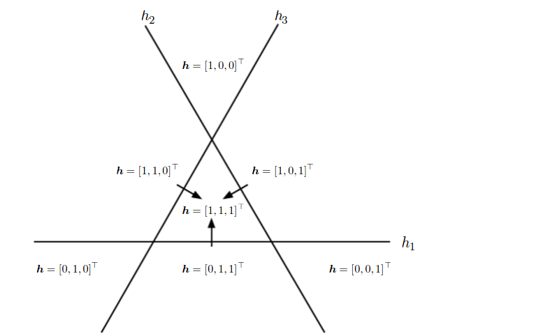
Actually, with a deeper representation you can approximate the same function and solve the same task more compactly, or solve more tasks with the same resources. For instance, traditional computer science studies Boolean circuits that implement or Boolean functions, and it turns out that many functions can be expressed much more efficiently if you allow for circuits of depth 3, some more functions, of depth 4, and so on, even though circuits of depth 2 can obviously express everything by reducing to a DNF or CNF. Something similar happens in machine learning. Picture a space of test points we want to sort into two groups. If we have only “one layer” then we can divide them with a (hyper)plane. If there are two layers then it comes down to linear separating surfaces composed of several hyperplanes (that’s roughly how boosting works — even very simple models become much more powerful if you compose them in the right way). On the third layer, yet more complicated structures made out of these separating surfaces take shape; it’s not all that easy to visualize them any more; and the same goes for subsequent layers. Below is a simple example from Goodfellow, Bengio, Courville “Deep Learning”. This illustration shows that if you combine even the simplest linear classifiers, each of which divides a plane into two half-planes, then, consequently, you can define regions of a much more complicated shape:
Thus, in deep learning we’re trying to build deeper architectures. We have described the main idea already — we pre-train the lower layers, one-by-one, and then finish training the whole network by finetuning with backpropagation. Therefore, let’s cover pretraining in more detail.
One of the simplest ideas is to train a neural network to copy its input to its output through a hidden layer. If the hidden layer is smaller, then it appears that the neural network should learn to extract some significant features from the data, which enables the hidden layer to restore the input. This type of neural network architecture is called an autoencoder. The simplest autoencoders are feedforward neural networks that are most similar to the perceptron and contain an input layer, hidden layer, and output layer. Unlike the perceptron, an autoencoder’s output layer has to contain as many neurons as its input layer.
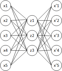
The training objective for this network is to bring theoutput vector x’ as close as possible to the input vector x
The main principle of (working with and) training an autoenconder network is to achieve a response on the output layer that is as close as possible to the input. Generally speaking, autoencoders are understood to be shallow networks, although there are exceptions.
Early autoencoders were basically doing dimensionality reduction. If you take much fewer hidden neurons than the inner and outer layers have, you wind up making the network compress the input into a compact representation, while at the same time ensuring that you’ll be able to decompress it later on. That’s what undercomplete autoencoders, where the hidden layer has lower dimension than the input and output layers, do. Now, however, overcomplete autoencoders are used much more often; they have a hidden layer of higher, sometimes much higher, dimension than that of the input layer. On the one hand, this is good, because you can extract more features. On the other hand, the network may learn to simply copy input to output with perfect reconstruction and zero error. To keep this from happening, you have to introduce regularization, not simply optimize the error.
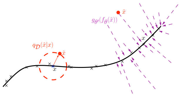
Returning the points to the dataset manifold
Classical regularization aims to avoid overfitting by using a prior distribution, like in a linear regression. But this won’t work in this case. Generally, autoencoders use more sophisticated methods of regularization that change inputs and outputs. One classical approach is a denoising autoencoder, which adds artificial noise to the input pattern and then asks the network to restore the initial pattern. In this case, you can make the hidden layer larger than that of the input (and output) layers: the network, however large, still has an interesting and nontrivial task to learn.
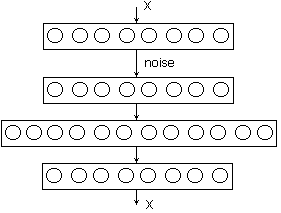
Incidentally, “noise” can be a rather radical change of the input. For instance, if it’s a binary pixel-based image then you can simply remove some of the pixels and replace them with zeroes (people often remove up to half of them!). However, the objective function you’re reconstructing is still the correct image. So, you make the autoencoder reconstruct part of the input based on another part. Basically, the autoencoder has to learn to understand how all the inputs are designed and understand the structure of the aforementioned manifold in a space with a ridiculous number of dimensions.
How deep learning works
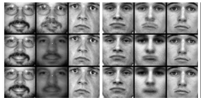
Suppose you want to find faces on pictures. Then one input data point is an image of a predefined size. Essentially, it’s a point in a multi-dimensional space, and the function you’re trying to find should take on the value of 0 or 1 depending on whether or not there’s a face on the picture. For example, mathematically speaking, a 4Mpix photo is a point in the space of dimension about 12 million: 4 million pixels times three color values per pixel. It’s glaringly obvious that only a small percentage of all possible images (points in this huge space) contain faces, and these images appear as tiny islands of 1s in an ocean of 0s. If you “walk” from one face to another in this multi-dimensional space of pixel-based pictures you’ll come across nonsensical images in the center; however, if you pre-train a neural network — by using a deep autoencoder, for instance — then closer to the hidden layer the original space of images turns into a space of features where peaks of the objective function are clustered much closer to one another, and a “walk” in the feature space will look much more meaningful.
Generally, the aforementioned approach does work; however, people can’t always interpret the extracted features. Moreover, many features are extracted by a conglomeration of neurons, which complicates matters. Naturally, one can’t categorically assert this is bad, but our modern notions of how the brain works tell us that different processes happen in the brain. We practically don’t have any dense layers, which means that only a small percentage of neurons responsible for extracting the features in question take part in solving each specific task.
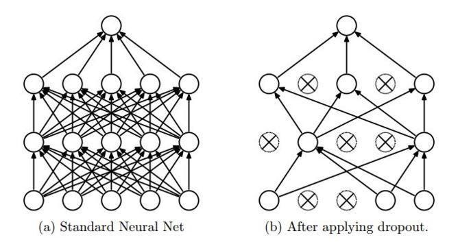
So how do you get each neuron to learn some useful feature? This brings us back to regularization; in this case, to dropout. As we already mentioned, a neural network usually trains by stochastic gradient descent, randomly choosing one object at a time from the training sample. Dropout regularization involves a change in the network structure: each node in the network is removed from training with a certain probability. By throwing away, say, half of the neurons, you get a new network architecture on every step of the training.
Having trained the other half of the neurons, we get a very interesting result. Now every neuron has to train to extract some feature by itself. It can’t count on teaming up with other neurons, because they may have been dropped out.
Dropout basically averages a huge number of different architectures. You build a new model on each test case. You take one model from this gigantic ensemble and perform one step of training, then you take another model for the next case and perform one step of training, and, eventually, you average all of these at the end, on the output layer. It is a very simple idea on the surface, but when dropout was introduced it led to great boons for practically all deep learning models.
We will go off on one more tangent that will link what’s happening now to the beginning of the article. What does a neuron do under dropout? It has a value, usually a number from 0 to 1 or from -1 to 1. A neuron sends this value further, but only 50% of the time rather than always. But what if we do it the other way around? Suppose a neuron always sends a signal of the same value, -namely ½, but sends it with probability equal to its value. The average output wouldn’t change, but now you get stochastic neurons that randomly send out signals. The intensity with which they do so depends on their output value. The larger the output the more the neuron is activated and the more often it sends signals. Does it remind you of anything? We wrote about that at the beginning of the article. That’s how neurons in the brain work. Like in the brain, neurons don’t transmit the spike’s amplitude, but rather they transmit one bit, the spike itself. It’s quite possible that our stochastic neurons in the brain perform the function of a regularizer, and it’s possible that, thanks to this, we can differentiate between tables, chairs, cats, and hieroglyphics.
After a few more tricks for training deep neural networks were added to dropout, it turned out that unsupervised pre-training wasn’t all that necessary, actually. In other words, the problem of vanishing gradients has mostly been solved, at least for regular neural networks (recurrent networks are a bit more complicated). Moreover, dropout itself has been all but replaced by new techniques such as batch normalization, but that would be a different story.
Sergey Nikolenko
Chief Research Officer, Neuromation
Leave a Reply