Category: Uncategorized

  • A Mixed Blessing I: Mixtures of Experts from Committee Machines to LLMs

    A Mixed Blessing I: Mixtures of Experts from Committee Machines to LLMs

    The world’s most powerful AI models are mostly asleep, just like our brains. Giant trillion-parameter models activate only a tiny fraction of their parameters for any given input, using mixtures of experts (MoE) to route the activations. MoE models began as a clever trick to cheat the scaling laws; by now, they are rapidly turning into the organizing principle of frontier AI models. In this post, we will discuss MoEs in depth, starting from the committee machines of the late 1980s and ending with the latest MoE-based frontier LLMs. We will mostly discuss LLMs and the underlying principles of MoE architectures, leaving vision-based and multimodal mixtures of experts for the second part.

    Introduction

    In December 2024, a relatively unknown Chinese AI lab called DeepSeek released a new model. As they say in Silicon Valley, it was a good model, sir. Their DeepSeek-V3 (DeepSeek AI, 2024), built with an architecture that has 671 billion parameters in total but activates only a fraction on each input, matched or exceeded the performance of models costing orders of magnitude more to train. One of their secrets was an architectural pattern that traces its roots back to the 1980s but has only recently become the organizing principle of frontier AI: Mixtures of Experts (MoE).

    If you have been following AI developments, you may have noticed a curious pattern. Headlines about frontier models trumpet ever-larger parameter counts: GPT-4’s rumored 1.8 trillion, Llama 4 Behemoth’s 2 trillion parameters. But these models are still quite responsive, and can be run efficiently enough to serve millions of users. What makes it possible is that frontier models are increasingly sparse. They are not monolithic neural networks where every parameter activates on every input. Instead, they are built on mixture of experts (MoE) architectures that include routing systems that dynamically assemble specialized components, activating perhaps only 10-20% of their total capacity for any given task.

    This shift from dense to sparse architectures may represent more than just an engineering optimization. It may be a fundamental rethinking of how intelligence should be organized—after all, biological neural networks also work in a sparse way, not every neuron in your brain fires even for a complex reasoning task. By developing MoE models with sparse activation, we can afford models with trillions of parameters that run on reasonable hardware, achieve better performance per compute dollar, and potentially offer more interpretable and modular AI systems.

    Yet the journey of MoEs has been anything but smooth. For decades, these ideas had been considered too complex and computationally intensive for practical use. It took many hardware advances and algorithmic innovations to resurrect them, but today, MoE architectures power most frontier large language models (LLMs). In this deep dive, we will trace this remarkable evolution of mixture of experts architectures from their origins in 1980s ensemble methods to their current status as the backbone of frontier AI.

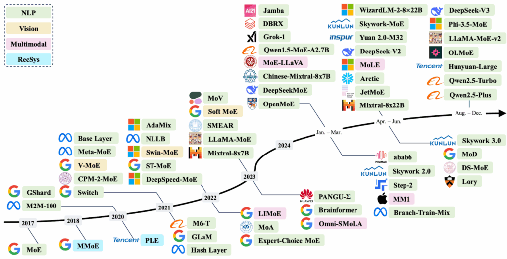
    Before we begin, let me recommend a few surveys that give a lot more references and background than I could here: Cai et al. (2024), Masoudnia, Ebrahimpour (2024), and Mu, Lin (2025). To give you an idea of the scale of these surveys, here is a general timeline of recent MoE models by Cai et al. (2024) that their survey broadly follows:

    Naturally, I won’t be able to discuss all of this in detail, but I do plan two posts on the subject for you, and both will be quite long. 

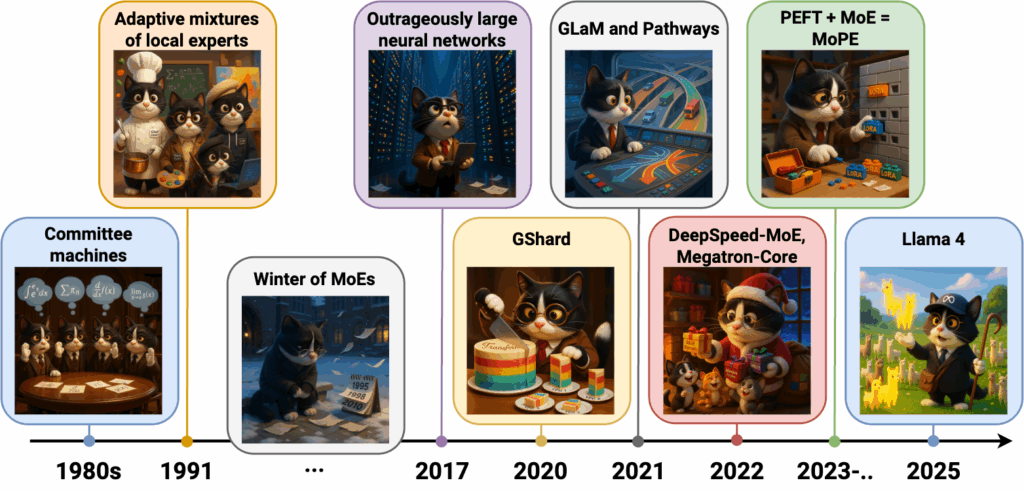
    In this first part, we discuss MoE architectures from their very beginnings in the 1980s to the latest LLMs, leaving the image processing and multimodal stuff for the second part. Here is my own timeline of the models and ideas and we touch upon in detail in this first part of the post; hopefully it will also serve as a plan for what follows:

    Let’s begin!

    MoE Origins: From Ensemble Intuition to Hierarchical Experts

    Despite their recent resurgence, mixtures of experts have surprisingly deep historical roots. To fully understand their impact and evolution, let us begin by tracing the origins of these ideas back to a much earlier and simpler era, long before GPUs and Transformer architectures started dominating AI research.

    Committee Machines (1980s and 1990s)

    The first appearance of models very similar to modern MoE approaches was, unsurprisingly, in ensemble methods, specifically in a class of models known as committee machines, emerging in the late 1980s and maturing through the early 1990s (Schwarze, Hertz, 1993; 1992).

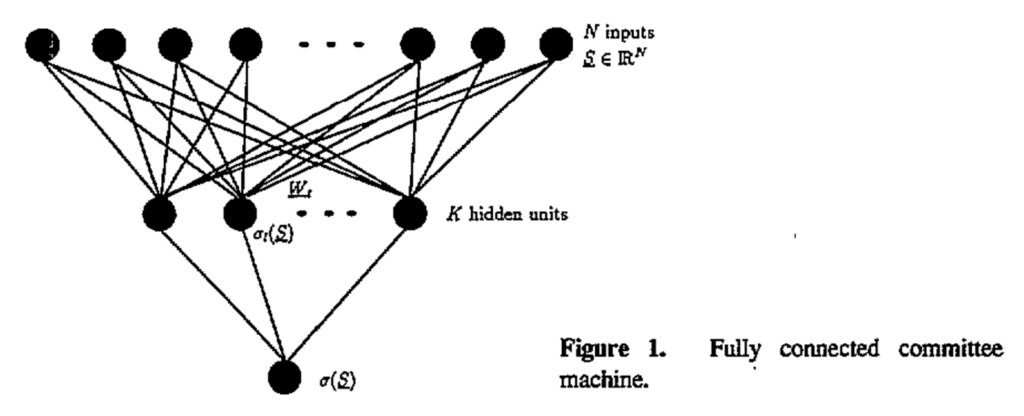
    These models combined multiple simple networks or algorithms—each independently rather weak—into a collectively strong predictor. Indeed, the boundary between committee machines and multilayered neural networks remained fuzzy; both combined multiple processing units, but committee machines emphasized the ensemble aspect while neural networks focused on hierarchical feature learning. For instance, here is an illustration by Schwarze and Hertz (1993) that looks just like a two-layered perceptron:

    Early theoretical explorations into committee machines applied insights from statistical physics (Mato, Parga, 1992), analyzing how multiple hidden units, called “committee members”, could collaboratively provide robust predictions.

    In their seminal 1993 work, Michael Perrone and Leon Cooper (the neurobiologist who was the C in BCM theory of learning in the visual cortex) demonstrated that a simple average of multiple neural network predictions could significantly outperform any single member. They found that ensembles inherently reduced variance and often generalized better, a cornerstone insight that I still teach every time I talk about ensemble models and committees in my machine learning courses.

    But while averaging neural networks was powerful, it was also somewhat naive: all ensemble members contributed equally regardless of context or expertise. A natural next step was to refine ensembles by letting each member specialize, focusing their attention on different parts of the input space. This specialization led to the key innovation behind mixtures of experts: gating mechanisms.

    First mixtures of experts (1991–1994)

    The first “true” MoE model was introduced in a seminal 1991 paper titled “Adaptive Mixtures of Local Experts” and authored by a very impressive team of Robert Jacobs, Michael Jordan, Steven Nowlan, and Geoffrey Hinton. They transformed the general notion of an ensemble into a precise probabilistic model, explicitly introducing the gating concept. Their architecture had a “gating network”, itself a neural network, that learned to partition the input space and assign inputs probabilistically to multiple “expert” modules:

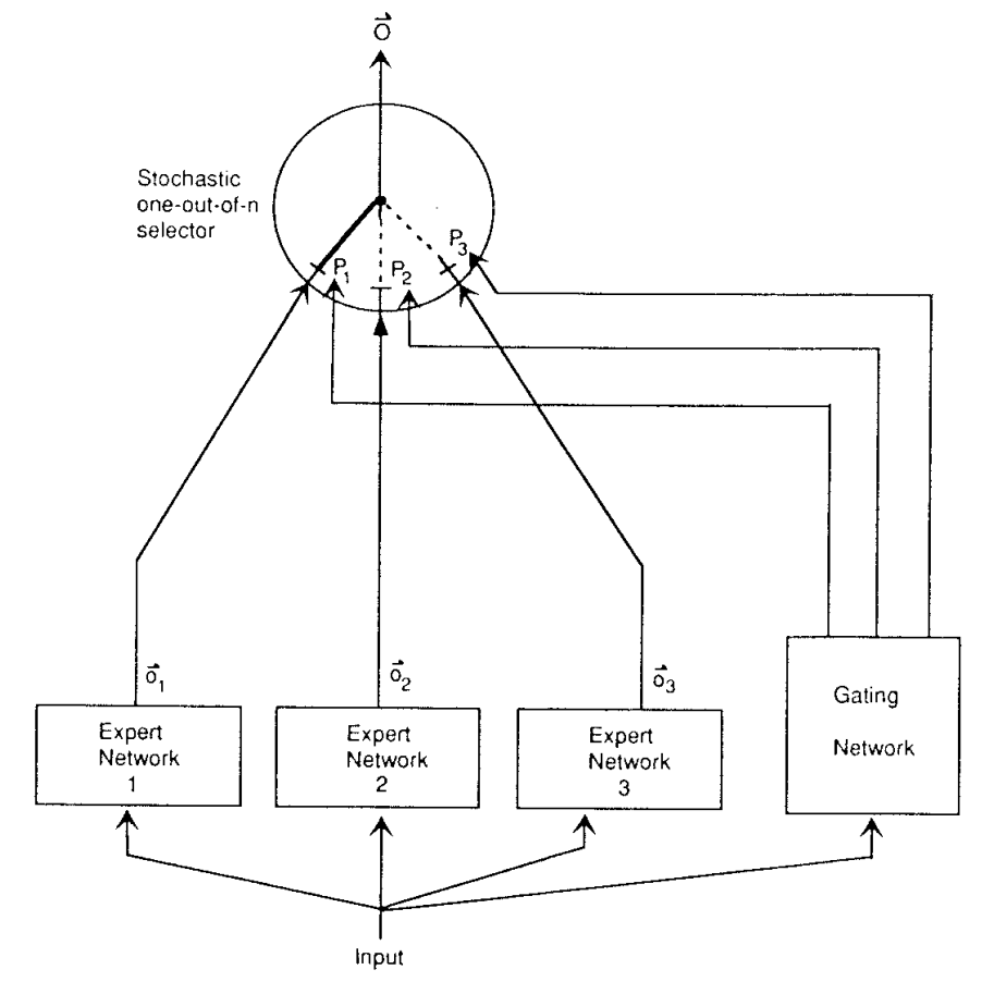
    Each expert would handle a localized subproblem, trained jointly with the gating network via gradient descent, minimizing the squared prediction error. Note that in the 1990s, every expert would be activated on every input, sparse gating would come much later.

    The follow-up work by Jordan and Jacobs extended this idea to hierarchical mixtures of experts (Jordan, Jacobs, 1991; 1993). Here, gating networks were structured into trees, where each node made a soft decision about passing data down one branch or another, progressively narrowing down to the most appropriate expert:

    Importantly, Jacobs and Jordan also saw how to apply the expectation-maximization (EM) algorithm for maximum likelihood optimization of these networks, firmly establishing MoE as a principled statistical modeling tool. EM is a very important tool in every machine learning researcher’s toolbox, appearing wherever models contain a lot of hidden (latent) variables, and hierarchical MoEs are no exception.

    In total, these seminal contributions introduced several fundamental concepts that are important for MoE architectures even today:

    • softmax gating probabilities, today mirrored as router logits in Transformer-MoE layers;
    • tree-structured gating networks, which are used in multi-layer or cascaded routing in modern implementations, and
    • Expectation-Maximization training, which keeps inspiring auxiliary losses in contemporary MoE implementations to balance expert load and ensure specialization;

    Moreover, back in the early 1990s the authors of these works also foresaw the benefits of modularity: experts could be independently updated, swapped, or fine-tuned; this is also widely used in today’s practice, as we will see below.

    The “winter of MoEs” (mid-1990s to 2010s)

    Given such promising beginnings, one might wonder why MoEs did not immediately revolutionize neural network research in the 1990s. Instead, mixtures of experts went through a period of dormancy lasting nearly two decades; they would resurface only in 2017.

    Why so? Mostly due to practical bottlenecks, most importantly high computational cost. The computers of the 1990s and early 2000s simply could not handle the parallel computation required to run many experts simultaneously. Typical experiments at that time involved small models even by the standards of the time, often with just a few thousand parameters in total, which did not let researchers exploit the scalability that is the main draw of MoEs.

    Besides, there were alternative methods readily available and actually working better. For instance, even the relatively narrow field of ensemble methods specifically were dominated by boosting approaches, starting from AdaBoost and later extended into gradient boosting methods. Boosting is indeed a better way to combine weak submodels, while MoEs begin to shine only as the component models become smarter.

    Nevertheless, some research continued. I want to highlight the Bayesian analysis of MoEs and hierarchical MoEs that was developed at the turn of the century (Jacobs et al., 1997; Bishop, Svenskn, 2002). By adding prior distributions to model parameters, Bayesian approaches helped address overfitting on smaller datasets and provided principled uncertainty estimates. These capabilities would prove valuable later when MoEs eventually scaled up, but for now, this theoretical groundwork laid dormant, waiting for the computational resources to catch up.

    There were also some practical applications in speech recognition (to model pronunciation variations) and computer vision (for fine-grained classification), but it was done at modest scale and without too much success. With the exception of the above-mentioned Bayesian analysis, MoEs remained largely absent from premier ML conferences.

    MoE Renaissance with Outrageously Large Networks

    Everything changed dramatically with the 2017 paper called “Outrageously Large Neural Networks” by Google Brain researchers Noam Shazeer et al. (again led by Geoffrey Hinton!). They revitalized mixtures of experts by creatively leveraging GPUs and introducing critical innovations.

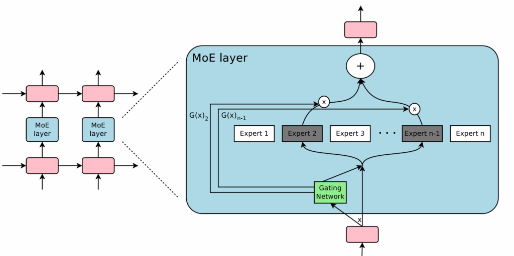
    The most important was the sparse gating mechanism: rather than activating every expert, they proposed to activate just the top-k experts (typically k=2) per input token, dramatically reducing computational overhead:

    Second, load-balancing auxiliary loss: to avoid the well-known “dead expert” problem (experts receiving zero or negligible input), they introduced a simple but effective auxiliary loss penalizing imbalanced usage across experts. Specifically, they introduced a smoothed version of the load function (probability that a given expert is activated under some random noise distribution) and a loss function that aims to reduce the coefficient of variation in the load.

    These improvements enabled Shazeer et al. to build a 137-billion-parameter MoE LSTM (in 2017, that was a huge, huge network!) that matched a dense LSTM with only 1 billion parameters in training costs, a spectacular scalability breakthrough. This work demonstrated how MoEs with conditional computation could efficiently scale to enormous sizes, and revitalized mixtures of experts for the ML community.

    The work by Shazeer et al. (2017) laid a foundation that modern MoE models have since built upon, inspiring large-scale implementations that we will discuss below. The underlying concepts—gating networks, localized specialization, and soft probabilistic routing—trace directly back to Jacobs and Jordan’s original formulations, but only with the computational power and practical innovations of recent years MoEs have been elevated from academic obscurity to practical prominence.

    Overall, in this section we have retraced the intellectual arc that led from committee machines in the late 1980s to modern trillion-parameter sparsely-gated transformers. Interestingly, many contemporary issues such as dead experts, router instability, and bandwidth bottlenecks were already foreseen in the early literature. If you read Jacobs and Jordan’s seminal papers and related early works carefully, you can still find valuable theoretical and practical insights even into today’s open problems.

    After this historical review, in the next sections we will go deeper into contemporary developments, starting with the remarkable journey of scaling language models with sparse conditional computation. Shazeer et al. used LSTM-based experts—but we live in the era of Transformers since 2017; how do they combine with conditional computation?

    Scaling Text Models with Sparse Conditional Compute

    If the historical journey of mixtures of experts (MoE) was a story of visionary ideas that could not be implemented on contemporary hardware, the next chapter in their story unfolded rapidly, almost explosively, once GPUs and TPUs arrived on the scene. By the early 2020s, scaling language models became the dominant focus of AI research. Yet, the push for ever-larger models soon faced both physical and economic limitations. Mixtures of experts, with their elegant promise of sparsity, offered a way around these limitations, and thus MoEs experienced a remarkable renaissance.

    GShard and Switch Transformer

    The era of modern MoE architectures began in earnest with Google’s GShard project in 2020 (Lepikhin et al., 2020). Faced with the huge Transformer-based models that already defined machine translation at that time, Google researchers looked for ways to train ultra-large Transformers without the typical explosive growth in computational costs. GShard’s key innovation was to combine MoE sparsity with Google’s powerful XLA compiler, which efficiently shards model parameters across multiple TPU devices.

    We are used to the idea that self-attention is the computational bottleneck of Transformers due to its quadratic complexity. However, for the machine translation problem Lepikhin et al. were solving, where the inputs are relatively short but latent dimensions are large, the complexity of a Transformer was entirely dominated by feedforward layers! For their specific parameters (d_{\mathrm{model}}=1024, d_{\mathrm{FF}}=8192, L=128 input tokens), a self-attention layer took 

        \[4\cdot L^2\cdot d_{\mathrm{model}} = 4\cdot 128^2 \cdot 1024 \approx 6.7\times 10^7 \text{ FLOPs},\]

    while a feedforward layer was ~32 times heavier with about

        \[2\cdot L\cdot d_{\mathrm{model}}\cdot d_{\mathrm{FF}} = 2\cdot 128 \cdot 1024 \cdot 8192\approx 2.15\times 10^9 \text{ FLOPs}.\]

    In terms of parameter count too, feedforward layers took about two thirds of a Transformer’s parameters (Geva et al., 2020). To put this in perspective: the self-attention computation was like calculating distances between 128 items, while the feedforward layer was like applying 8192 different transformations to each item—a much heavier operation.

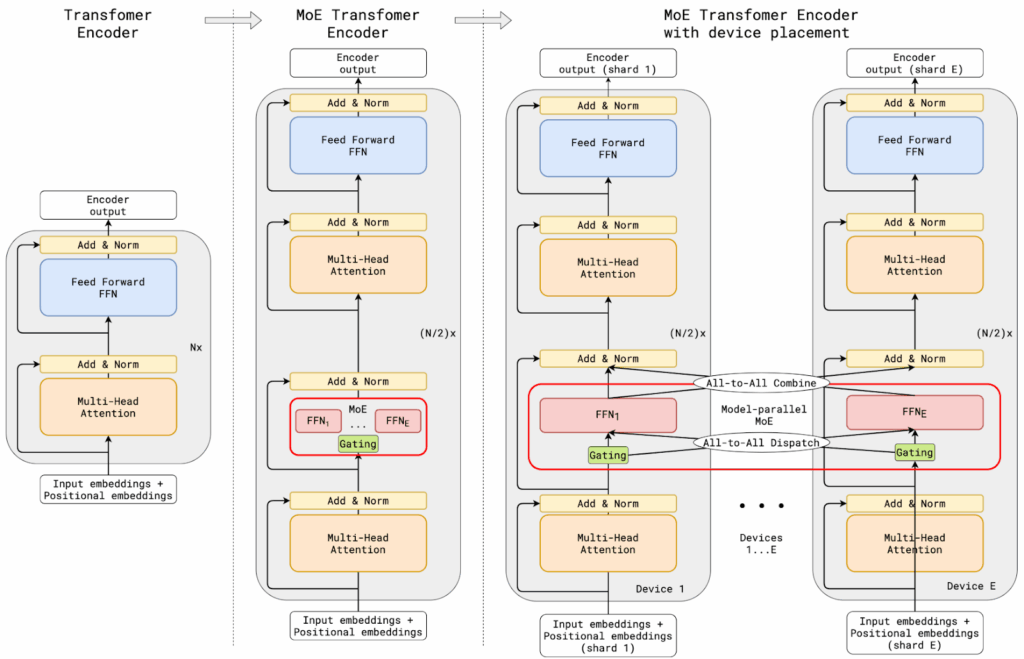
    So the approach of Lepikhin et al. (2020) was concentrated on feedforward layers. Instead of each Transformer block performing a single dense computation, they replaced half of the dense feed-forward layers with sparsely gated mixture of experts layers (the illustration shows that only every other FF layer is turned into a MoE layer):

    The gating mechanism selectively activates only a handful of experts per input token, thus dramatically reducing the computational load. Gating also included load balancing, this time for training: each expert was assigned a “capacity” value, and on every mini-batch, the number of tokens assigned to an expert cannot exceed this capacity. Lepikhin et al. (2020) also introduced a highly parallel implementation for a cluster of TPUs, which was also very helpful, although perhaps too technical to discuss here.

    This allowed GShard to reach previously unattainable scales; ultimately, they trained a 600-billion-parameter machine translation model on 2,048 TPUs over just four days. Moreover, this model delivered a substantial improvement in machine translation metrics compared to dense baselines at similar computational cost.

    Another Google Brain project, this time by Fedus et al. (2021), introduced the Switch Transformer in early 2021. Building directly on GShard’s sparse routing idea, the Switch Transformer took sparsity to a more extreme form, implementing a “top-1 routing” mechanism. In GShard, two experts handled each token (unless their capacity was exceeded or one of them had a low weight), but Switch Transformer simplified matters further by activating only the single most appropriate expert per token. Again, this idea was applied to feedforward layers:

    This simplification ran contrary to contemporary sensibilities: Shazeer et al. (2017) hypothesized that you have to compare several (at least two) experts to have nontrivial signal for the routing function, and other works studied the number of experts required and found that more experts were helpful, especially in lower layers of the network (Ramachandran, Le, 2018).

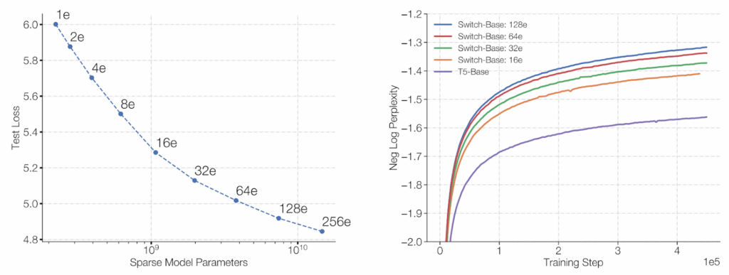
    Still, Fedus et al. (2021) proved to be right: switching worked just as well as regular gating, only faster. The Switch Transformer was the first to successfully train a model with a trillion parameters! Even more importantly, increasing the number of parameters in this sparse setting still conformed to the famous scaling laws of Kaplan et al. (2020) and allowed training to be much more sample-efficient, i.e., achieve the same results with less data and training compute:

    The Switch Transformer emphatically proved that MoE models could not only scale but also remain stable, trainable, and economical. But machine translation was just the beginning.

    GLaM and the Pathways approach

    Inspired by the groundbreaking successes of GShard and Switch Transformer, later in 2021 Google Research introduced the Generalist Language Model (GLaM; Du et al., 2022), a further improved MoE-based sparse architecture. 

    Similar to GShard, GLaM replaces every other Transformer layer with a MoE layer, and at most two experts are activated for every input. But they added recent modifications that the original Transformer architecture had received by that time—Gated Linear Units in feedforward layers (Shazeer, 2020) and GELU activations (Hendrycks, Gimpel, 2016)—and utilized even more aggressive sparsity, activating only 8% of its 1.2 trillion parameters per token. This resulted in GLaM outperforming GPT-3 in both results and computational costs, and in a scaling law that held at least up to 64 experts:

    Despite this extreme sparsity, GLaM performed very well on benchmark tasks, often matching or surpassing dense models such as GPT-3 (175B parameters), while using only a fraction (about one-third) of the energy during training.

    GLaM was not just a single model with a novel technical breakthrough; it represented a philosophical shift. Google’s broader “Pathways” initiative introduced soon after (Dean, 2021) contained a vision of single models capable of handling multiple tasks and modalities efficiently by selectively activating different parts of the network—pathways—based on context:

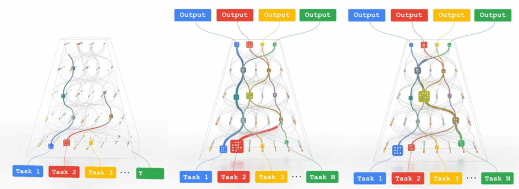
    The vision already suggested hierarchical routing strategies, where one router would select broad modality-specific pathways and another would pick fine-grained token-level experts, just like modern multimodal architectures such as Gemini 1.5 do.

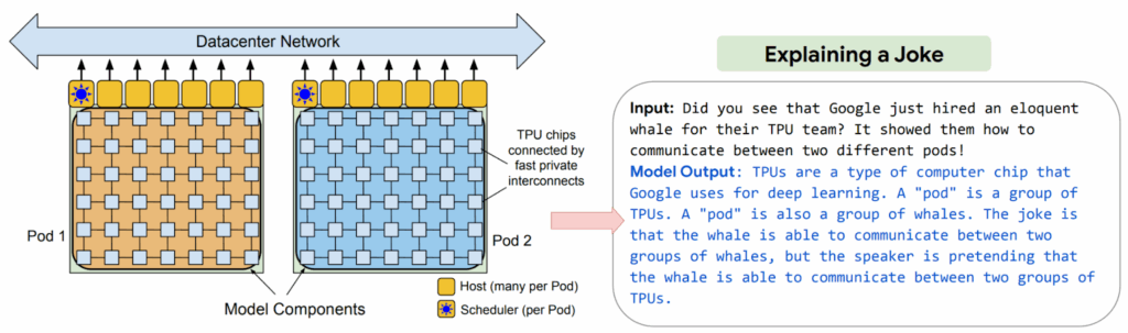
    The first widely adopted result of this initiative was the Pathways Language Model (PaLM)  LLM released by Google in April 2022 (Chowdhery et al., 2022). While PaLM itself was not a MoE model, it represented Google’s commitment to the broader Pathways vision of conditional computation and served as an important stepping stone towards their later MoE implementations in Gemini. Where GLaM/MoE models saved compute by explicitly sparse activations, PaLM showed that a dense Transformer could still scale to half-a-trillion params if the communication stack is re-engineered. Specifically, PaLM used a client-server graph and gradient exchange between denser compute clusters to achieve near-linear throughput, scaling for the first time to two TPU pods… which let PaLM understand jokes about pods much better:

    PaLM also popularized chain-of-thought prompting, showing how asking the model to generate its reasoning consistently boosts results across multiple applications. It became a popular and important family of LLMs, leading to PaLM 2 (Anil et al., 2023) and specialized offshoots such as Med-PaLM for medical applications (Singhal et al., 2023a; 2023b) and PaLM-E for embodied reasoning (Driess et al., 2023).

    Note that PaLM is not a mixture-of-experts model per se, it is a dense model where every layer is activated on every input. To be honest, it’s not really a full implementation of the Pathways idea either; it runs on the Pathways orchestration level but does not employ the original detailed routing idea. As Chowdhery et al. (2022) put it themselves, “PaLM is only the first step in our vision towards establishing Pathways as the future of ML scaling at Google and beyond”.

    Still, it was a great first step and an important stepping stone towards distributed LLM architectures. But when and how did actual MoE models enter the frontier LLM landscape? While PaLM demonstrated the power of dense models with novel distributed orchestration, the fundamental efficiency gains of sparse architectures were still underexplored. Let us see how two major industry players took up the challenge of making MoE models practical and ready for widespread adoption.

    DeepSpeed-MoE and Megatron-Core: opensourcing MoE for the masses

    In 2022, the landscape of LLMs was not yet as firmly established as today, where new entries such as Grok require huge investments from the richest guys in the world and still kind of fall short. The DeepSpeed family and its Megatron offshoots could try to come anew and define the LLM frontier.

    Although, to be fair, there were not one, but two extremely rich companies involved: DeepSpeed was developed by Microsoft researchers, while the Megatron family was trained with the vast computational resources of NVIDIA. They first came together to produce the Megatron-Turing Natural Language Generation model (MT-NLG), which had a record-breaking 530B parameters back in October 2021 and broke a lot of records in natural language understanding and generation tasks (Smith et al., 2022; Kharya, Alvi, 2021).

    By mid-2022, both teams of researchers tried to build on this success with sparse architectures. DeepSpeed-MoE (Rajbhandari et al., 2022) set the goal to make mixture of experts models practical for GPT-style language modelling, i.e., cheap to train and, crucially, cheap to serve in production. The paper presents an end-to-end stack that includes new architecture tweaks, compression ideas, distributed training, and an inference engine.

    They use top-1 gating (already standard when you want to be fast and cheap), still sparsify only the feedforward parts of the Transformer architecture, and shard each expert into its own GPU rank, mixing data and tensors so that every GPU processes exactly one expert. 

    The MoE architectural novelty in DeepSpeed-Moe was the Pyramid-Residual MoE (PR-MoE). The pyramid part means that early layers keep fewer experts, and later layers double them, which reflects the idea that deeper layers learn task-specific concepts. The residual part means that each token always passes through a small dense MLP branch, while the expert acts as a residual “error-corrector”:

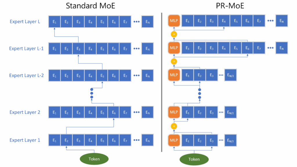
    This allowed DeepSpeed-MoE to have up to 3x fewer parameters with virtually identical zero-shot accuracy.

    Another interesting trick was about the distillation process that could train smaller MoE ensembles that approach the quality of the original much larger variant. Rajbhandari et al. (2022) noticed that while distillation is a natural idea for MoE models as well (although it was still novel at the time—Artexte et al., 2021 and Fedus et al., 2022 distilled MoE models before, but only into dense smaller Transformers), it starts to hurt the results after a while if you just distill larger experts into smaller ones. Thus, they introduced Mixture-of-Students (MoS) distillation: the student experts copy the teacher for the first 40% of pretraining, and then distillation is turned off so the students can keep minimizing their own LM loss.

    All of these innovations—and many more—have made their way into an open source release. The DeepSpeed library, still supported and improved by Microsoft researchers, emerged as a very influential open source framework. For MoE models specifically, it offers CUDA kernels optimized for sparsity together with sophisticated memory management techniques, and later developed DeepSpeed’s ZeRO-3 memory partitioning method (from Zero Redundancy Optimizer, first introduced by Rajbhandari et al., 2019; see also ZeRO++ by Wang et al., 2023) further pushed scalability, allowing massive MoE models to run on relatively modest hardware configurations.

    NVIDIA’s Megatron-LM suite, which includes the Megatron-Core framework with MoE implementations, followed shortly thereafter, introducing specialized kernels known as Grouped-GEMM, which efficiently batch many small expert computations into a single GPU operation. Megatron-Core also pioneered capacity-aware token dropping and systematic monitoring tools to alleviate common MoE issues like dead experts. These innovations significantly streamlined training pipelines, accelerating adoption of MoE at scale across diverse applications. What’s more, the Megatron-LM suite is also published in open source and has become the basis for many interesting research advances (Shoeybi et al., 2019; Shin et al., 2020; Boyd et al., 2020; Wang et al., 2023; Waleffe et al., 2024).

    While DeepSpeed and Megatron showed that it was feasible to scale MoEs up, the real test would come with their adoption in production systems serving millions of users. In the next section, we will examine how today’s frontier LLMs have embraced and extended these ideas. Are state of the art LLMs powered by MoEs or have they found a better way to scale?

    Mixtures of Experts in Flagship LLMs

    Actually, the answer is yes. Between 2023 and 2025, MoE architectures firmly transitioned from research artifacts to production-ready frontier models. Let me show three prominent models that exemplify this shift.

    Mixtral of Experts

    It is fashionable to frown upon Mistral AI, a European research lab whose top models indeed often do not match the best American and Chinese offerings in scale and capabilities, and the EU AI Act and other associated bureaucracy is not helping matters.

    But they are committed to open source, where they make significant contributions to the field, and the Mixtral family rapidly became an open-source sensation in 2023. Specifically, we are interested in the Mixtral of Experts idea (Jiang et al., 2024; Mistral AI, 2023) and its 8x7B model based on the Mistral-7B backbone (Jiang et al., 2023) that has entered plenty of baseline comparisons and has given rise to a lot of research papers. 

    Mixtral 8x7B is relatively small: 47B total parameters with 13B of them active per token, 32 layers with 8 experts per layer and top-2 routing, and only 32K tokens of context. The MoE implementation is straightforward—when a token arrives at a feedforward layer (again, here we leave the self-attention layers unchanged), a router scores it into 8 logits, only the top 2 survive, and their outputs are combined in a linear combination:

    Unlike previous MoE architectures, Mixtral 8x7B has small fan-out (only 8 experts) but top-2 routing instead of the common top-1 choice; this seems to provide a better quality-compute trade-off, and 13B active parameters fit on commodity GPUs, so many researchers could run Mixtral 8x7B for their projects without huge funding.

    The Mistral AI team also studied which experts get activated for which tokens. 

    And here is an illustration of which experts get activated on which tokens for several layers in the architecture (Jiang et al., 2024); note that it’s less semantic and perhaps more syntactic than you would expect, especially at top layers:

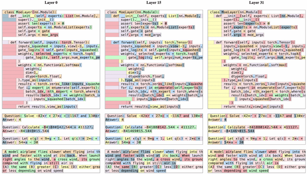
    With good clean multilingual training data, Mixtral 8x7B became the first open-source MoE that rivaled GPT-3.5 on average while running on a single GPU.

    Gemini 1.5 Pro

    Google’s flagship model, Gemini 1.5 (Gemini Team, 2024), showcased multimodal routing across text, images, audio, and video, delivering previously unimaginable context windows—up to an astonishing 10 million tokens.

    Again, Gemini 1.5 Pro replaces most of the dense feed-forward blocks with MoE blocks, routing every token to a small subset of experts. The main difference from previous MoE iterations was that previously MoE LLMs were unimodal, topped out at 2–32K tokens of context, and their expert routing was still fairly simple. Gemini 1.5 introduces a multimodal encoder-decoder, raises the context size up to millions of tokens, and introduces a more careful gating scheme (materials mention DSelect-k by Hazimeh et al., 2021, which we will discuss below), so load balancing stays healthy even when the prompt is a 700K-token codebase.

    Gemini also introduced intricate caching strategies, such as cross-expert KV-cache sharing, which led to significant gains in cost efficiency and, again, context enlargement.

    GPT-4 and later OpenAI models

    OpenAI is notoriously not that open with its research ideas (and perhaps they are quite correct in that!), so I cannot really tell you what were the novelties of GPT-4o in detail; all we have officially are the system cards for GPT-4 (OpenAI, 2023) and GPT-4o (OpenAI, 2024), which are both mostly about capabilities and safety rather than about the ideas. So the following details should be taken as informed speculation rather than confirmed facts.

    But there have been leaks and analyses, and I can link to a Semianalysis post on GPT-4 that suggests that GPT-4o (and its base model GPT-4) employs approximately 16 experts per MoE layer, each with around 111 billion parameters, amounting to roughly 1.8 trillion total parameters with around 280 billion active at any given time; see also here and here.

    While the exact number of parameters may be different, it’s almost certain that starting from GPT-4, OpenAI’s latest models are all of the MoE variety. This lets them both be huge and at the same time have reasonable runtimes. GPT-4 routes to the top 2 experts out of 16, and there are, it seems, specialized experts fine-tuned to do specific stuff, e.g., one expert concentrates on safety and another on coding. GPT-4o seems to have the same basic structure but several efficiency improvements that are about, e.g., sparse attention mechanisms rather than MoE.

    Note that GPT-4 is still the workhorse of the latest reasoning models such as o4-mini, o3 and o3-pro; the release of a larger model, GPT-4.5 (OpenAI, 2025), was not that successful, and while I cannot be 100% sure it seems like all top OpenAI’s offerings are still GPT-4-powered.

    DeepSeek-V3

    The Chinese top tier model, DeepSeek-V3 (DeepSeek AI, 2024), which soon became the basis for the famous DeepSeek-R1 reasoning model (Guo et al., 2025), pushes breadth: lots of fine-grained experts, relatively large K, sophisticated router engineering to keep them busy, and a lot of very insightful tricks in the training process to make the giant 671B parameter model as efficient as possible. Here let me refer to my previous longform post where I went into some details about the engineering ingenuity of DeepSeek-V3.

    Llama 4

    Probably the latest frontier family of models that we do have detailed information about is the Llama 4 family, introduced in April 2025 (Meta AI, 2025). And fortunately for us now, instead of using a dense decoder-only transformer like the Lllama 3 family, Llama 4 became the first of the Llama models to implement a MoE-based architecture.

    For example, the Llama 4 Maverick model employs a large MoE architecture with 128 experts per layer and top-2 routing, meaning that each token activates 2 experts out of 128. The total parameter count reaches over 400 billion, but only about 17B parameters are active per token, making it efficient to run. One of these two experts in the Llama 4 family is a shared expert:

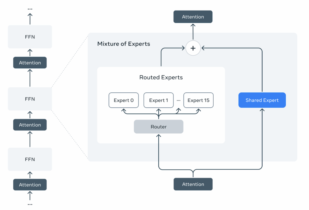
    The model also introduced several innovations in the Transformer architecture itself, in particular the iRoPE approach with interleaved attention layers without positional embeddings. Perhaps most importantly for the open-source community, Meta released not just the model weights (on Huggingface) but also detailed training recipes and infrastructure code (on GitHub), making it a great starting point for others to train their own MoE models at scale.

    With that, we are already basically at the frontier of modern LLMs; latest improvements deal with fine-tuning strategies and turning one-shot LLMs into reasoning models, which do not change the underlying model structure. So let me end the high-level survey part of the post here and proceed to actually diving into the details of routing strategies and other architectural choices that a MoE model designer has to make.

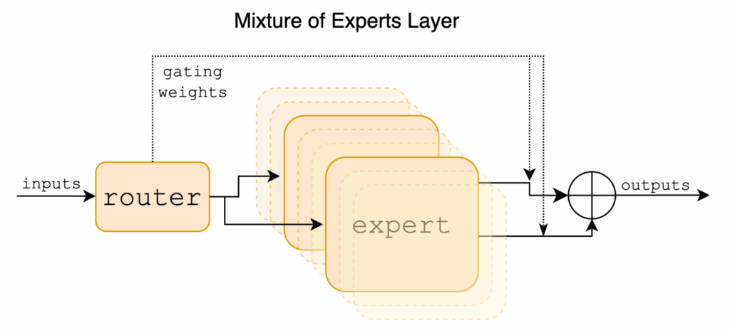
    Router Mechanics: How To Train Your Monster

    Mixtures of experts sound very simple from a bird’s eye view: you have lots of small, specialized networks (“experts”), and for every input, you activate just a few, as chosen by a router which is also a subnetwork. But translating this elegant idea into reality involves many important practical considerations. How exactly do routers work? What other considerations are there? In this section, let’s dive beneath the surface and explore exactly how engineers tame this beast in practice.

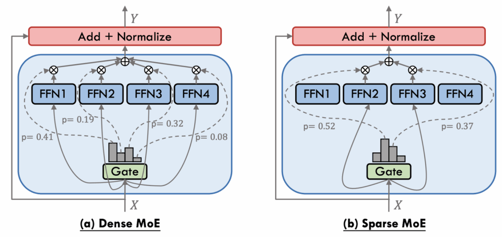
    Sparse vs. dense MoEs

    The first important distinction is between dense and sparse MoEs: do we combine the experts in a full linear combination or do we choose a small subset of the expert? Here is an illustration by Cai et al. (2024):

    Formally speaking, a dense MoE router produces some vector of scores \mathbf{g}(\mathbf{x},\boldsymbol{\theta}), where \boldsymbol{\theta} are the router’s parameters and \mathbf{x} is the input, and then uses it as softmax scores:

        \[F(\mathbf{x},\boldsymbol{\theta},\mathbf{W})=\sum_{i=1}^n\mathrm{softmax}\left(g(\mathbf{x},\boldsymbol{\theta})\right)\cdot f_i(\mathbf{x},\mathbf{w}_i),\]

    where \mathbf{w}_i are the weights of the experts. A sparse MoE router only leaves the top k of these scores and sets the rest to negative infinity so that the softmax would lead to zero probabilities:

        \[g_{i,\mathrm{sparse}}(\mathbf{x},\boldsymbol{\theta})=\mathrm{TopK}(\mathbf{g}(\mathbf{x},\boldsymbol{\theta}))_i=\begin{cases} g_i(\mathbf{x},\boldsymbol{\theta}), & \text{if it is in the top }k, \\-\infty, & \text{otherwise}.\end{cases}\]

    Early works mostly used dense MoEs (Jordan, Jacobs, 1991; 1993; Collobert et al., 2001). But ever since GShard that we discussed above (Shazeer et al., 2017) had introduced and popularized sparse routing, it was the common agreement that sparse routing is the way to go as a much more efficient solution: you don’t have to activate all experts every time. 

    The only remnants of dense MoEs were shared experts, pioneered by the DeepSpeed-MoE (Rajbhandari et al., 2022) architecture that we discussed above. In this case, every token is processed by a fixed expert (which is “densely activated”, so to speak) and another expert chosen through gating, so it is actually top-1 gating with two resulting experts.

    It has been known that dense MoEs might work better—see, e.g., Riquelme et al. (2021)—but the tradeoff has been generally assumed to be not worth it. Still, interestingly, work on dense mixtures of experts has not stopped, and sometimes it has been very fruitful. Let me highlight a few of these cases; they are very different but each explores alternatives to the classical sparsely-gated Top-k MoE layer.

    EvoMoE (Evolutional Mixture-of-Experts; Nie et al., 2021) introduces two-phase training. On the expert-diversify phase, they start with one shared expert, then copy and randomly mask it to spawn many diverse experts. On the gate-sparsify phase, they introduce the Dense-to-Sparse (DTS) gate: a softmax that initially routes tokens to all experts but then gradually prunes itself until it behaves like a sparse Top-1 or Top-2 routing gate. Here is an illustration by Nie et al. (2021):

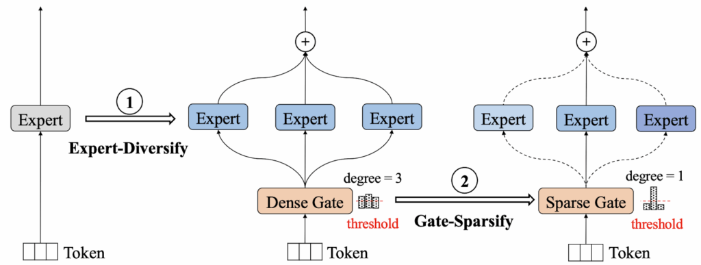
    As a result, routing is fully dense at the beginning, allowing every expert to receive gradient signals; sparsity is imposed only after experts have specialized, so in this case the authors try to get the best of both worlds with a hybrid training procedure.

    MoLE (Mixture of LoRA Experts; Wu et al., 2024) notices that sparseness is important when experts are large, but there are use cases when they aren’t. What if your experts are LoRA adapters? Then you can treat every independently trained LoRA as an expert and learn a hierarchical soft-max gate that mixes them layer-by-layer.

    The idea is to get an economical but expressive way to learn to adaptively combine different LoRAs; here is a comparison vs. linear composition (left) and reference tuning (center), two other popular methods for LoRA composition:

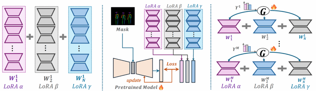
    Moreover, because the routing gate is continuous, MoLE can later mask unwanted experts at inference time and renormalize weights without retraining. Wu et al. (2024) introduce a gating balance loss that keeps experts alive and avoids dominance by a few adapters. As a result, they get an approach that can scale to dozens of adapters with little extra memory because only the tiny routing gate is trainable.

    Another creative way to combine LoRA adapters with a MoE mechanism was introduced in LoRAMoE (Dou et al., 2024). Compared to standard MoE, LoRAMoE replaces each feedforward layer by a mini-MoE whose experts are low-rank LoRA matrices; the output is a dense weighted sum over all experts:

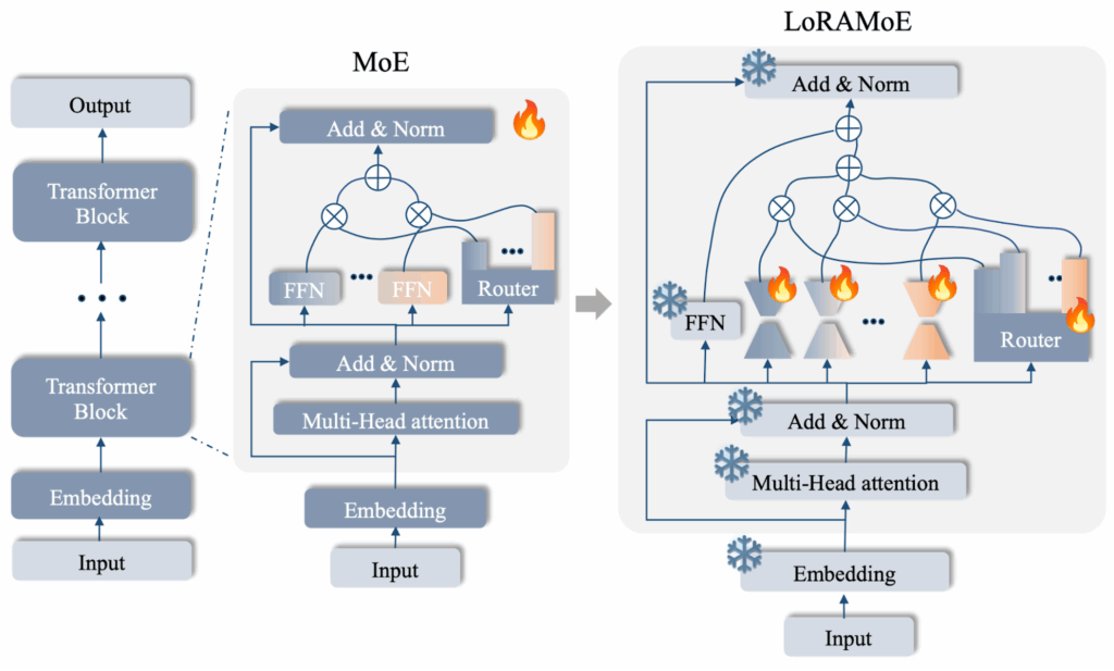
    Basically, just freeze the backbone, plug in multiple LoRA adapters as experts and blend them with a dense router. Moreover, Dou et al., (2024) specialize their experts explicitly, introducing a localized balancing constraint that biases half of the experts towards knowledge-heavy tasks and half towards instruction following (we are talking about image-to-text models here).

    Interestingly, they applied it to LLMs and found that dense MoE and a frozen backbone preserve pretrained world knowledge much better than full SFT or single-LoRA tuning. After fine-tuning on specific downstream tasks, the LoRAMoE architecture lost much less performance on general question answering benchmarks about the world than the alternatives.

    As you can see, sparse vs. dense MoE is not a dichotomy but more of a spectrum: you can switch between pure dense and pure sparse MoE in training, or apply dense MoEs to smaller subnetworks, or use any other hybrid approach that might be preferable in your specific case.

    MoPE and where to place it

    The discussion of MoLE and LoRAMoE brings us to a whole different class of MoE-based architectures: Mixtures of Parameter-Efficient Experts (MoPE). MoPE is a design paradigm that combines two ideas that had previously advanced largely in parallel:

    • the conditional computation and specialization benefits of MoEs and
    • the memory- and compute-friendly techniques of parameter-efficient fine-tuning (PEFT) such as LoRA, conditional adapters, prefix tuning and others (see, e.g., a detailed survey by Han et al., 2024).

    In MoPE, the heavy dense backbone of a pretrained LLM is frozen, and each expert represents a lightweight PEFT module. A gating network selects, per token or per example, the subset of PEFT experts that will be applied on top of the frozen weights. The idea is to combine the task-adaptivity and routing diversity of MoEs while not actually spending the storage and FLOPs budget usually associated with sparse expert layers. It was pioneered by MoELoRA (Liu et al., 2023) and MixLoRA (Li et al., 2024) and has blossomed into a subfield of its own.

    Since we are talking about PEFT now, there is a wide variety of different places where one can put the adapter inside a standard Transformer stack of the base model. Here I will again use an illustration by Cai et al. (2024) with a general taxonomy of these placements, and then we will consider them one by one:

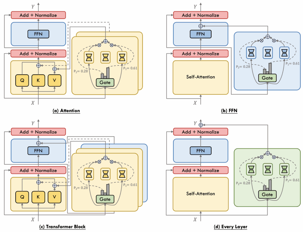
    In attention-level MoPE, experts augment individual projection matrices (Q, K, V, O). E.g., MoELoRA (Liu et al., 2023) inserts multiple LoRA experts into the Query and Value projections and uses top-k routing plus a contrastive loss to encourage expert diversity and stable routing. MoCLE (Gou et al., 2024) clusters tasks first and then routes inputs to cluster-specific LoRA experts plus a universal backup expert.

    FFN-level MoPE adapts the feedforward sublayer, as classical MoEs usually do, but instead of gating the full FFN parallel PEFT experts are added and combined through gating. AdaMix (Wang et al., 2022) pioneered this setting, using adapter experts with a stochastic routing policy at training time that collapses to a cheap ensemble at inference, while MixDA (Diao et al., 2023) places domain-adapters and task-adapters sequentially to disentangle domain and task knowledge. LoRAMoE (Dou et al., 2024) that we have discussed above also belongs to this class.

    In Transformer-block-level MoPE, two expert pools are attached simultaneously—one modulating the self-attention block, the other the FFN. For example, MoV (Zadouri et al., 2024) replaces both blocks’ dense parameters with tunable vectors, showing large memory savings without sacrificing quality, while MoLoRA from the same work follows the dual-pool idea but sticks to LoRA experts. UniPELT (Mao et al., 2024) mixes heterogeneous PEFT methods (adapter, prefix, LoRA) under separate gates, letting the model pick the most suitable adaptation mechanism per input.

    Finally, layer-wise (or every-layer) MoPE treats the entire Transformer layer as the unit of specialization, with each layer hosting a set of PEFT experts applied to the whole block.  We have discussed MoLE (Wu et al., 2024) that views already-trained LoRAs as ingredients and learns only the gating weights to compose them on-the-fly for a new domain. Omni-SMoLA (Wu et al., 2024) extends the idea to three modality-specific expert sets (text, vision, and multimodal) for vision-and-language tasks.

    Training regimes

    Another design choice that a MoE system has to make is how exactly to train the experts. Early MoE systems such as GShard and Switch Transformer simply replaced each feed-forward block with a sparse MoE layer and trained the entire network end-to-end; inference mirrored the training configuration without architectural changes. This approach remains a standard baseline, but by now there are three major routes that one can follow to try and improve upon it.

    Dense-to-sparse regime starts with a dense backbone and gradually introduces sparsity.  For example, Residual MoE (RMoE; Wu et al., 2022) pretrains a Vision Transformer densely, then fine-tunes it with sparsely activated experts while aligning outputs between the original FFN and the emerging MoE layer. EvoMoE (Nie et al., 2021) that we have discussed above bootstraps knowledge with a single expert, then spawns additional experts, and employs a Dense-to-Sparse Gate (DTS-Gate) that performs gradual annealing from full activation to top-k routing, thus alleviating the cold start problems for experts. The Sparse Upcycling approach (Komatsuzaki et al., 2023) copies FFN weights from a well-trained dense checkpoint into multiple identical experts, adds a randomly initialized router, and then retrains the network. DS-MoE (Pan et al, 2024) and SMoE-Dropout (Chen et al., 2023) are hybrid approaches that alternate between dense and sparse activations during training so that all experts receive gradient signal (this is needed to avoid expert under-utilization), but inference reverts to sparse execution for efficiency.

    Sparse-to-dense distillation or pruning aims for deployability: how do we compress a high-capacity sparse MoE into a latency-friendly dense model. For example, Switch Transformer (Fedus et al., 2021) distills knowledge into a dense student with only ~5% of the parameters, while OneS (Xue et al., 2023) first aggregates expert weights by SVD or top-k heuristics, then distills into a single dense model that can keep 60–90 % of the parent’s gains across vision and NLP tasks. ModuleFormer (Shen et al., 2023) and Expert-Slimming / Expert-Trimming strategies by He et al. (2024) prune under-used experts or average their weights back into a single FFN, yielding a structurally dense network that preserves most task accuracy while significantly reducing memory and communication costs. In general the Sparse-to-Dense training mode demonstrates that MoE can serve as a training scaffold: once knowledge has diversified across experts, it can be re-fused into a compact model without full retraining.

    Finally, expert-model merging means that experts are trained independently and then fused together with a router. For example, the Branch-Train-Merge (BTM; Li et al., 2022) and Branch-Train-MiX (BTX; Sukhbaatar et al., 2024) pipelines train several dense experts independently on domain-specific data and later fuse their FFNs into a single MoE layer, leaving attention weights averaged. Then MoE is briefly fine-tuned in order to teach the router to exploit this cross-domain complementarity. The Fusion of Experts (FoE; Wang et al., 2024) framework generalizes this idea, treating merging as supervised learning over heterogeneous expert outputs. Expert-model merging avoids the heavy communication of joint MoE training and allows recycling of preexisting specialist checkpoints, which is particularly attractive when there are external reasons against combined training such as, e.g., privacy concerns.

    Obviously, the dimensions of sparse vs. dense routing, PEFT placement, and training modes are orthogonal, and there have been plenty of different variations for each of these ideas; let me again link to the surveys here (Cai et al., 2024; Masoudnia, Ebrahimpour, 2024; Mu, Lin, 2025). Moreover, these are not even the only dimensions. One could also consider different ways to feed training data or different engineering approaches to sharding the experts on a computational cluster and organizing communication between them. But I hope that this section has given you a good taste of the diversity of MoE approaches, and perhaps we will investigate some other dimensions in the second part.

    Conclusion

    The journey of mixtures of experts has been a journey from relatively obscure ensemble methods that couldn’t quite find a good problem fit to the backbone of frontier AI systems. This evolution offers several important lessons about innovation in machine learning and points toward some future directions.

    First, timing matters as much as brilliance. The core MoE ideas from Jacobs et al. (1991) were essentially correct—they just arrived twenty-five years too early. Without GPUs, distributed computing, and modern optimization techniques, even the most elegant algorithms remained academic curiosities. This pattern repeats throughout ML history. For example, the main ideas of Transformer architectures were arguably already introduced in the attention mechanisms of the early 1990s but needed computational scale to shine, diffusion models had spent years in relative obscurity before efficient sampling algorithms were developed, and reinforcement learning required massive simulation infrastructure to tackle large-scale problems. The lesson for researchers is both humbling and hopeful: your “failed” idea might just be waiting for its technological moment, and also, perhaps, we will hear more about other “failed” ideas in the future, when the time is right.

    Second, sparsity is not just an optimization trick—it is an important design principle. The success of MoE models demonstrates that by activating only 1-10% of parameters per input, we can achieve what dense models cannot: gracefully scale to trillions of parameters while maintaining reasonable inference costs. This sparse activation pattern mirrors biological neural networks, where specialized regions handle specific functions, and human organizations, where human experts collaborate dynamically based on a specific task. Perhaps the future of AI lies not in ever-larger monolithic models but in large ecosystems of specialized components, assembled on-demand for each specific problem.

    Third, the best architectures balance elegance with engineering. Every successful MoE implementation requires both theoretical insights and pragmatic engineering; we have talked about the former in this first part, and next time we will talk some more about the latter.

    In the second part of this mini-series, we will explore how these same MoE principles are transforming computer vision and multimodal AI, where the routing problem becomes even more fascinating: how do you decide which experts should handle a pixel, a word, or the boundary between them? The principles we have explored—sparse activation, specialized expertise, dynamic routing—take on new dimensions when applied across modalities. Stay tuned!

    Sergey Nikolenko
    Head of AI, Synthesis AI

  • Synthetic Data: The Early Days, Part I

    Synthetic Data: The Early Days, Part I

    Previously on this blog, we have discussed the data problem: why machine learning may be hitting a wall, how one-shot and zero-shot learning can help, how come reinforcement learning does not need data at all, and how unlabeled datasets can inform even supervised learning tasks. Today, we begin discussing our main topic: synthetic data. Let us start from the very beginning: how synthetic data was done in the early days of computer vision…

    A brief intro to synthetic data

    Let me begin by reminding the general pipeline of most machine learning model development processes:

    Synthetic data is an important approach to solving the data problem by either producing artificial data from scratch or using advanced data manipulation techniques to produce novel and diverse training examples. The synthetic data approach is most easily exemplified by standard computer vision problems, and we will do so in this post too, but it is also relevant in other domains.

    In basic computer vision problems, synthetic data is most important to save on the labeling phase. For example, if you are solving the segmentation problem it is extremely hard to produce correct segmentation masks by hand. Here are some examples from the Microsoft COCO (Common Objects in Context) dataset:

    You can see that the manually produced segmentation masks are rather rough, and it is very expensive to make them much better if you need a large-scale dataset as a result.

    But suppose that all these scenes were actually 3D models, rendered in virtual environments with a 3D graphics engine. In that case, we wouldn’t have to painstakingly label every object with a bounding box or, even worse, a full silhouette: every pixel would be accounted for by the renderer and we would have all the labeling for free! What’s more, the renderer would provide useful labeling which is impossible for humans and which requires expensive hardware to get in reality, such as, e.g., depth maps (distance to camera) or surface normals. Here is a sample from the ProcSy dataset for autonomous driving:

    We will speak a lot more about synthetic data in this blog, but for now let us get on to the main topic: how synthetic data started its journey and what its early days looked like.

    The first steps: line drawings as synthetic data

    Computer vision started as a very ambitious endeavour. The famous “Summer Vision Project” by Seymour Papert was intended for summer interns and asked to construct a segmentation system, in 1966:

    Back in the 1960s and 1970s, usable segmentation on real photos was very hard to achieve. As a result, people turned to… synthetic data! I am not kidding, synthetic images in the form of artificial drawings are all over early computer vision.

    Consider, for example, the line labeling problem: given a picture with clearly depicted lines, mark which of the lines represent concave edges and which are convex. Here is a sample picture with this kind of labeling for two embedded parallelepipeds, taken from the classic paper by David Huffman, Impossible Objects as Nonsense Sentences:

    Figure (a) on the left shows a fully labeled “X-ray” image, and figure (b) shows only the visible part, but still fully labeled. And here is an illustration of a similar but different kind of labeling, this time from another classic paper by Max Clowes, On Seeing Things:

    Here Clowes distinguishes different types of corners based on how many edges form them and what kind of edges (concave or convex) they are. So basically it’s the same problem: find out the shape of a polyhedron defined as a collection of edges projected on a plane, i.e., shown as a line drawing.

    Both Huffman and Clowes work (as far as I understand, independently) towards the goal of developing algorithms for this problem. They address it primarily as a topological problem, use the language of graph theory and develop conditions under which a 2D picture can correspond to a feasible 3D scene. They are both fascinated with impossible objects, 2D drawings that look realistic and satisfy a lot of reasonable necessary conditions for realistic scenes but at the same time still cannot be truly realized in 3D space. Think of M.C. Escher’s drawings (on the left, a fragment from “Ascending and descending”) or the famous Penrose triangle (on the right):

    And here are two of the more complex polyhedral shapes, the one on the left taken from Huffman and on the right, from Clowes. They are both impossible but it’s not so easy to spot it by examining local properties of their graphs of lines:

    But what kind of examples did Huffman and Clowes use for their test sets? Well, naturally, it proved to be way too hard for the computer vision of the 1960s to extract coherent line patterns like these from real photographs. Therefore, this entire field was talking about artificially produced line drawings, one of the first and simplest examples of synthetic data in computer vision.

    Synthetic data for a quantitative comparison

    In the early days of computer vision, many problems were tackled not by machine learning but by direct attempts to develop algorithms for specific tasks. Let us take as the running example the problem of measuring optical flow. This is one of the basic low-level computer vision problems: estimate the distribution of apparent velocities of movement along the image. Optical flow can help find moving objects on the image or estimate (and probably subtract) the movement of the camera itself, but its most common use is for stereo matching: by computing optical flow between images taken at the same time from two cameras, you can match the picture in stereo and then do depth estimation and a lot of scene understanding. In essence, optical flow is a field of vectors that estimate the movement of every pixel between a pair of images. Here is an example (taken from here):

    The example above was produced by the classical Lucas-Kanade flow estimation algorithm. Typical for early computer vision, this is just an algorithm, there are no parameters to be learned from data and no training set. In their 1981 paper, Lucas and Kanade do not provide any quantitative estimates for how well their algorithm works, they just give several examples based on a single real world stereo pair. Here it is, by the way:

    And this is entirely typical: all early works on optical flow estimation develop and present new algorithms but do not provide any means for a principled comparison beyond testing them on several real examples.

    When enough algorithms had been accumulated, however, the need for an honest and representative comparison became really pressing. For an example of such a comparison, we jump forward to 1994, to the paper by Barron et al. called Performance of Optical Flow Techniques. They present a taxonomy and survey of optical flow estimation algorithms, including a wide variety of differential (such as Lucas-Kanade), region-based, and energy-based methods. But to get a fair experimental comparison, they needed a test set with known correct answers. And, of course, they turned to synthetic data for this. They concisely sum up the pluses and minuses of synthetic data that remain true up to this day:

    The main advantages of synthetic inputs are that the 2-D motion fields and scene properties can be controlled and tested in a methodical fashion. In particular, we have access to the true 2-D motion field and can therefore quantify performance. Conversely, it must be remembered that such inputs are usually clean signals (involving no occlusion, specularity, shadowing, transparency, etc.) and therefore this measure of performance should be taken as an optimistic bound on the expected errors with real image sequences.

    For the comparison, they used sinusoidal inputs and a moving dark square over a bright background:

    They also used synthetic camera motion: take a still real photograph and start cropping out a moving window over this image, and you get a camera moving perpendicular to its line of sight. And if you take a window and start expanding it, you get a camera moving outwards:

    These synthetic data generation techniques were really simple and may seem naive by now, but they did allow for a reasonable quantitative comparison: it turned out that even on such seemingly simple inputs the classical optical flow estimation algorithms gave very different answers, with widely varying accuracy.

    Conclusion

    Today, we saw two applications of synthetic data in early computer vision. First, simple line drawings suffice to present an interesting challenge for 3D scene understanding, even when interpreted as precise polyhedra. Second, while classical algorithms for low-level computer level problems almost never involved any learning of parameters, to make a fair comparison you need a test set with known correct answers, and this is exactly where machine learning can step up. But stay tuned, that’s not all, folks! See you next time!

    Sergey Nikolenko
    Head of AI, Synthesis AI

  • NeuroNuggets: Cut-and-Paste in Deep Learning

    NeuroNuggets: Cut-and-Paste in Deep Learning

    …Many people think that authors
    just cut and paste from real life into books.
    It doesn’t work quite that way.
    ― Paul Fleischman

    As the CVPR in Review posts (there were five: GANs for computer visionpose estimation and tracking for humanssynthetic datadomain adaptation, and face synthesis) have finally dried up, we again turn to our usual stuff. In the NeuroNugget series, we usually talk about specific ideas in deep learning and try to bring you up to speed on each. We have had some pretty general and all-encompassing posts here, but it is often both fun and instructive to dive deeper into something very specific. So we will devote some NeuroNuggets to reviewing a few recent papers that share a common thread.

    And today, this thread is… cut-and-paste! And not the kind we all do from other people’s GitHub repositories. In computer vision, this idea is often directly related to synthetic data, as cutting and pasting sometimes proves to be a fertile middle ground between real data and going fully synthetic. But let’s not get ahead of ourselves…

    Naive Cut-and-Paste as Data Augmentation

    We have talked in great detail about object detection and segmentation, two of the main problems of computer vision. To solve them, models need training data, the more the merrier. In modern computer vision, training data is always in short supply, so researchers always use various data augmentation techniques to enlarge the dataset.

    The point of data augmentation is to introduce various modifications of the original image that do not change the ground truth labels you have or change them in predictable ways. Common augmentation techniques include, for instance, moving and rotating the picture and changing its color histogram in predictable ways:

    Image source

    Or changing the lighting conditions and image parameters that basically reduce to applying various Instagram filters:

    Image source

    Notice how in terms of individual pixels, the pictures change completely, but we still have a very predictable and controllable transformation of what the result should be. If you know where the cat was in the original image, you know exactly where it is in the rotated-and-cropped one; and Instagram filters usually don’t change the labels at all.

    Data augmentation is essential to reduce overfitting and effectively extend the dataset for free; it is usually silently understood in all modern computer vision applications and implemented in standard deep learning libraries (see, e.g., keras.preprocessing.image).

    Cutting and pasting sounds like a wonderful idea in this regard: why not cut out objects from images and paste them onto different backgrounds? The problem, of course, is that it is hard to cut and paste an object in a natural way; we will return to this problem later in this post. However, last year (2017) has seen a few papers that claimed that you don’t really have to be terribly realistic to make the augmentation work.

    The easiest and most straightforward approach was taken by Rao and Zhang in their paper “Cut and Paste: Generate Artificial Labels for Object Detection” (appeared on ICVIP 2017). They simply took an object detection dataset (VOC07 and VOC12), cut out objects according to their ground truth labels and pasted them onto images with different backgrounds. Like this:

    Source: (Rao, Zhang, 2017)

    Then they trained with these images, using cut-and-paste like usual augmentation. Even with this very naive approach, they claimed to noticeably improve the results of standard object detection networks like YOLO and SSD. More importantly, they claimed to reduce common error modes of YOLO and SSD. The picture below shows the results after training on the left; and indeed, wrong labels decrease and bounding boxes significantly improve in many cases:

    Source: (Rao, Zhang, 2017)

    A similar but slightly less naive approach to cutting and pasting was introduced, also in 2017, by researchers from the Carnegie Mellon University. In “Cut, Paste and Learn: Surprisingly Easy Synthesis for Instance Detection” (ICCV 2017), Dwibedi et al. use the same basic idea but instead of just placing whole bounding boxes they go for segmentation masks. Here is a graphical overview of their approach:

    Source: (Dwibedi et al., 2017)

    Basically, they take a set of images of the objects they want to recognize, collect a set of background scenes, and then paste objects into the scene. Interestingly, they are recognizing grocery items in indoor environments, just like we did in our first big project on synthetic data.

    Dwibedi et al. claim that it is not really important to place objects in realistic ways globally but important to achieve local realism. That is, modern object detectors do not care as much to have a Coke bottle on the counter rather than on the floor; however, it is important to blend the object as realistically as possible into the local background. To this purpose, Dwibedi et al. consider several differ blending algorithms for pasting images:

    Source: (Dwibedi et al., 2017)

    They then make blending another dimension of data augmentation, another factor of variability in order to make the detector robust against boundary artifacts. Together with other data augmentation techniques, it proves highly effective; “All Blend” in the table below means that all versions of blending for the same image are included in the training set:

    Source: (Dwibedi et al., 2017)

    This also serves as evidence for the point about the importance of local realism. Here are some sample synthetic images Dwibedi et al. come up with:

    Source: (Dwibedi et al., 2017)

    As you can see, there is indeed little global realism here: objects are floating in the air with no regard to the underlying scene. However, here is how the accuracy improves when you go from real data to real+synthetic:

    Source: (Dwibedi et al., 2017)

    Note that all of these improvements have been achieved in a completely automated way. The only thing Dwibedi et al. need to make their synthetic dataset is a set of images for that would be easy to segment (in their case, they have photos of objects on a plain background). Then it is all in the hands of neural networks and algorithms: a convolutional network predicts segmentation masks, an algorithm does augmentation for the objects, and then blending algorithms make local patches more believable, so the entire pipeline is fully automated. Here is a general overview of what algorithms constitute this pipeline:

    Source: (Dwibedi et al., 2017)

    Smarter Augmentation: Pasting with Regard to Geometry

    We have seen that even very naive pasting of objects can help improve object detection by making what is essentially synthetic data. The next step in this direction would be to actually try to make the pasted objects consistent with the geometry and other properties of the scene.

    Here we begin with a special case: text localization, i.e., object detection specifically for text appearing on an image. That is, you want to take a picture with some text on it and output bounding boxes for the text instances regardless of their form, font, and color, like this:

    Image source

    This is a well-known problem that has been studied for decades, but here we won’t go into too many details on how to solve it. The point is, in 2016 (the oldest paper in this post, actually) researchers from the University of Oxford proposed an approach to blending synthetic text into real images in a way coherent with the geometry of the scene. In “Synthetic Data for Text Localisation in Natural Images”, Gupta et al. use a novel modification of a fully convolutional regression network (FCRN) to predict bounding boxes, but the main novelty lies in synthetic data generation.

    They first sample text and a background image (scraped from Google Image Search, actually). Then the image goes through several steps:

    • first, through a contour detection algorithm called gPb-UCM; proposed in (Arbelaez, Fowlkes, 2011), it does not contain any neural networks and is based on classical computer vision techniques (oriented gradient of histograms, multiscale cue combination, watershed transform etc.), so it is very fast to apply but still produces results that are sufficiently good for this application;
    • out of the resulting regions, Gupta et al. choose those that are sufficiently large and have sufficiently uniform textures: they are suitable for text placement;
    • to understand how to rotate the text, they estimate a depth map (with a state-of-the-art CNN), fit a planar facet to the region in question (with the RANSAC algorithm), and then add the text, blending it in with Poisson editing.

    Here is a graphical overview of these steps, with sample generated images on the bottom:

    Source: (Gupta et al., 2016)

    As a result, Gupta et al. manage to produce very good text placement that blends in with the background scene; their images are not realistic only in the sense that we might not expect text to appear in these places at all, otherwise they are perfectly fine:

    Source: (Gupta et al., 2016)

    With this synthetic dataset, Gupta et al. report significantly improved results in text localization.

    In “Synthesizing Training Data for Object Detection in Indoor Scenes”, Georgakis et al. from the George Mason University and University of North Carolina at Chapel Hill applied similar ideas to pasting objects into scenes rather than just text. Their emphasis is on blending the objects into scenes in a way consistent with the scene geometry and meaning. To do this, Georgakis et al.:

    • use the BigBIRD dataset (Big Berkeley Instance Recognition Dataset) that contains 600 different views for every object in the dataset; this lets the authors blend real images of various objects rather than do the 3D modeling required for a purely synthetic approach;
    • use an approach by Taylor & Cowley (2012) to parse the scene, which again uses the above-mentioned RANSAC algorithm (at some point, we really should start a NonNeuroNuggets series to explain some classical computer vision ideas — they are and will remain a very useful tool for a long time) to extract the planar surfaces from the indoor scene: counters, tables, floors and so on;
    • combine this extraction of supporting surfaces with a convolutional network by Mousavian et al. (2012) that combines semantic segmentation and depth estimation; semantic segmentation lets the model understand which surfaces are indeed supporting surfaces where objects can be placed;
    • then depth estimation and positioning of the extracted facets are combined to understand the proper scale and position of the objects on a given surface.

    Here is an illustration of this process, which the authors call selective positioning:

    Source: (Georgakis et al., 2017)

    Here (a) and (e) show the original scene and its depth map, (b) and © show semantic segmentation results with predictions for counters and tables highlighted on (c), (f) is the result of plane extraction, and (g) are estimated supporting surfaces; they all combine to find regions for object placement shown on (d), and then the object is properly scaled and blended on (h) to obtain the final result (i). Here are some more examples to show that the approach indeed works quite well:

    Source: (Georgakis et al., 2017)

    Georgakis et al. train and compare Faster R-CNN and SSD with their synthetic dataset. Here is one of the final tables:

    Source: (Georgakis et al., 2017)

    We won’t go into the full details, but it basically shows that, as always, you can get excellent results on synthetic data by training on synthetic data, which is useless, and you don’t get good results on real data by training purely on this kind of synthetic data. But if you throw together real and synthetic then yes, there is a noticeable improvement compared to using just the real dataset. Since this is still just a form of augmentation and thus is basically free (provided that you have a dataset of different views of your objects), why not?

    Cutting and Pasting for Segmentation… with GANs

    Finally, the last paper in our review is a quite different animal. In this paper recently released by Google, Remez et al. (2018) are actually solving the instance segmentation problem with cut-and-paste, but they are not trying to prepare a synthetic dataset to train a standard segmentation model. Rather, they are using cut-and-paste as an internal quality metric for segmentations: a good segmentation mask will produce a good image with a pasted object. In the image below, a bad mask (a) leads to an unconvincing image (b), and a good mask (c) produces a much better image (d), although the ground truth (e) is better still:

    Source: (Remez et al., 2018)

    How does the model decide which images are “convincing”? With an adversarial architecture, of course! In the model pipeline shown below, the generator is actually doing the segmentation, and the discriminator judges how well the pasted image is by trying to distinguish it from real images:

    Source: (Remez et al., 2018)

    The idea is simple and brilliant: only a very good segmentation mask will result in a convincing fake, hence the generator learns to produce good masks… even without any labeled training data for segmentation! The whole pipeline only requires the bounding boxes for objects to cut out.

    But you still have to paste objects intelligently. There are several important features required to make this idea work. Let’s go through them one by one.

    1. Where do we paste? One can either paste uniformly at random points of the image or try to take into account the scene geometry and be smart about it, like in the papers above. Here, Remez et al. find that yes, pasting objects in a proper scale and place in the scene does help. And no wonder; in the picture below, first look on the left and see how long it takes you to spot the pasted objects. Then look on the right, where they have been pasted uniformly at random. Where will the discriminator’s job be easier?

    Source: (Remez et al., 2018)

    2. There are a couple of degenerate corner cases that formally represent a very good solution but are actually useless. For example, the generator could learn to “cut off” all or none of the pixels in the image and thus make the result indistinguishable from real… because it is real! To discourage from choosing all pixels, the discriminator simply receives a larger viewpoint, seeing, so to speak, the bigger picture, so this strategy ceases to work. To discourage from choosing no pixels, the authors introduce an additional classification network that attempts to classify the object of interest and the corresponding loss function. Now, if the object has not been cut, classification will certainly fail, incurring a large penalty.

    3. Sometimes, cutting only a part of the segmentation mask still results in a plausible object. This is characteristic for modular structures like buildings; for example, in these satellite images some of the masks are obviously incomplete but the resulting cutouts will serve just fine:

    Source: (Remez et al., 2018)

    To fix this, the authors set up another adversarial game, now trying to distinguish the background resulting from cutting out the object and the background resulting from the same cut elsewhere in the scene. This is basically yet another term in the loss function; modern GANs often tend to grow pretty complicated loss functions, and maybe someday we will explore them in more details.

    The authors compare their resulting strategy with some other pretrained baselines; while they, of course, lose to fully supervised methods (with access to ground truth segmentation masks in the training set), they come out ahead against the baselines. It is actually pretty cool that you can get segmentation masks like this with no effort for segmentation type labeling:

    Source: (Remez et al., 2018)

    There are failure cases too, of course. Usually they happen when the result is still realistic enough even with the incorrect mask. Here are some characteristic examples:

    Source: (Remez et al., 2018)

    This work is a very interesting example of a growing trend towards data-independent methods in deep learning. More and more often, researchers find ways around the need to label huge datasets, and deep learning gradually learns to do away with the hardships of data labeling. We are not quite there yet but I hope that someday we will be. Until next time!

    Sergey Nikolenko
    Chief Research Officer, Neuromation

  • Neuromation Team in Singapore

    Neuromation Team in Singapore

    This week we start our Asian Road show, with the first stop in Singapore! Yesterday, Neuromation team had an AI & Blockchain Meetup at Carlton Hotel.

    We have met AI enthusiasts, researchers, developers and innovators, telling them more about what is AI, Machine Learning, Deep Learning, Neural Networks and how is AI being applied to improve our world, our businesses, and our lives.

    Our team-members, Dr. Sergey Nikolenko, Mr. Maksym Prasolov, Mr. Evan Katz, Mr. Arthur McCallum and Mr. Daniel Liu told about Neuromation case and the future of AI.

    Neuromation Road Show continues, come and meet us at the AI Expo at Tokyo Big Sight, April 4th-6th, at the booth 4–7!

  • AI in Biology and Medicine

    AI in Biology and Medicine

    Today I present to you three research directions that apply the latest achievements in artificial intelligence (mostly deep neural networks) to biomedical applications. Perhaps, this is the research that will not only change but also significantly extend our lives. I am grateful to my old friend, co-author, and graduate student Arthur Kadurin who has suggested some of these projects.

    Translated from Russian by Andrey V. Polyakov. Original article here.

    Polar, Beyersdorf AG, and Others: Smart Clothes

    We begin with a series of projects that are unlikely to turn the world over but will certainly produce, pardon the pun, cosmetic changes in everyday life already in the nearest future. These projects deal with AI applications for the so-called “Internet of Things” (IoT), specifically applications that are very “close to the body”.

    Various types of fitness trackers, special bracelets that collect information about heartbeat, steps, and so forth, have long ago entered our life. The main trend at the sportswear companies now is to build different sensors directly into the clothes. That way, you can collect more information and measure it more precisely. Sensors suitable for “smart clothes” were invented in 2016, and already in 2017 Polar has presented Polar Team Pro Shirt, a shirt that collects lots of information during exercises. The plot will no doubt thicken even further when sports medicine supported by artificial intelligence will learn to use all this information properly; I expect a revolution in sports that Moneyball could never dream of.

    And it is already beginning. Recently, on November 24–26, the second SkinHack hackathon dedicated to applying machine learning models to analyzing data coming from such sportswear took place in Moscow. The first SkinHack held last year was dedicated to “smart cosmetics”; the participants tried to predict the age of a person by the skin structure on photographs looking for wrinkles. Both smart cosmetics and smart clothing are areas of active interest for Beiersdorf AG (commonly known as the producer of the Nivea brand), so one can hope that the commercial launch of these technologies will be not long in coming. In Russia, SkinHack was supported by Youth Laboratories, a company affiliated with the central characters of our next part…

    Insilico: Automatic Discovery of New Drugs

    Insilico Medicine is a company well known in the biomedical world. Its primary mission is to fight aging, and I personally wish Insilico success in this effort: one does not look forward to growing old. However, in this article I would like to emphasize another, albeit related, project of the company: drug discovery based on artificial intelligence models.

    A medicinal drug is a chemical compound that can link with other substances in our body (usually proteins) and have the desired effect on them, e.g., suppress a protein or start producing another in larger quantities. To find a new drug, you need to choose from a huge number of possible chemical compounds exactly the ones that will have the desired effect.

    It is clear that at this point it is impossible to fully automate the search for new drugs: clinical trials are needed, and one usually starts testing on mice, then on humans… in general, the process of bringing a new medicinal drug to the market usually takes years. However, one can try to help doctors by reducing the search space. Insilico develops machine learning models that try not only to predict the properties of a molecule but also to generate candidate molecules with desired properties, thereby helping to choose the most promising candidates for further laboratory and clinical studies.

    This search space reduction is done with a very interesting class of deep learning models: generative adversarial networks (GAN). Such networks combine two components: a generator trying to generate new objects — for example, new molecules with desired properties — and a discriminator trying to distinguish generated results from real data points. Learning to deceive the discriminator, the generator begins to generate objects indistinguishable from the real ones… that is, hopefully, actually real ones in this case. The last Insilico model, called druGAN (drug + GAN), attempts to generate, among others, molecules useful for oncological needs.

    MonBaby: Keeping Track of the Baby

    Finally, I would like to end with a project that Neuromation plans to participate in. Small children, especially babies, cannot always call for help themselves and require special care and attention. This attention is sometimes required even in situations where mom and dad seem to be able to relax: for example, a sleeping baby may hurt a leg by turning to an uncomfortale pose . And then there is the notorious SIDS (sudden baby death syndrome), whose risk has been linked with the pose of a sleeping infant: did you know that the risk of SIDS increases several times if a baby sleeps on the stomach?

    The MonBaby smart infant tracking system is a small “button” that snaps onto clothing and monitors the baby’s breathing and turning around while asleep. Currently, the system is based on machine learning for time series analysis: data from baby movements is used to recognize breathing cycles and sleeping body position (on the stomach or on the back).

    We plan to complement this system with smart cameras able to track the infant’s movements and everything that happens to him or her by visual surveillance. The strong suits of our company will come in handy here: computer vision systems based on deep convolutional networks and synthetic data for their training. The fact is that in this case it is practically impossible to collect a sufficiently large real data set for training the system: it would take not only real video recordings of tens of thousands of babies, but video recordings with all possible critical situations. Thankfully, modern ethics, both medical and human, would never allow us to generate such datasets in real life. Therefore, we plan to create “virtual babies”, 3D models that will allow us to simulate the necessary critical situations and generate synthetic videos for training.

    We have briefly examined three directions in different branches of biomedicine — sports medicine and cosmetics, creating medicines and baby care — each of which is actively using the latest achievements of artificial intelligence. Of course, these are just examples: AI is now used in hundreds of diverse biomedical projects (which we may touch upon in later articles). Hopefully, however, with these illustrations I have managed to show how AI research is working on helping people live longer, better, and healthier.

    Sergey Nikolenko,
    Chief Research Officer, Neuromation

  • AI: Should We Fear The Singularity?

    AI: Should We Fear The Singularity?

    Source: https://www.if24.ru/ai-opasna-li-nam-singulyarnost/

    Recently, discussions on artificial intelligence (AI) in popular publications have become increasingly alarmist. Some are trying to prove that AI will oust 90% of live people from the market, condemning them to unemployment and misery. Others go even further, asking whether the humankind can find in strong artificial intelligence an existential risk that no hydrogen bomb can match. Let us try to find out.

    Supporters of treating AI as an existential risk usually mean the “intelligence explosion” scenario, when a powerful AI acquires a capability to improve itself (for example, by rewriting parts of the code), thereby becoming even “smarter”, which allows for even more radical improvements, and so forth. More details about this can be found in the AI-Foom debate between Robin Hanson and Eliezer Yudkowsky, a very interesting read that discusses this exact scenario. The main danger here is that the goals of the resulting superhuman artificial intelligence may not really align to the goals and original intentions of its human creators. A common example in the field goes as follows: if the original task of a powerful AI was something as innocent as producing paperclips, in a week or two after the “intelligence explosion” the Earth might find itself completely covered by fully automated factories of two kinds: factories producing paperclips and factories for constructing spaceships to bring paperclip manufacturing factories to other planets…

    Such a scenario does sound upsetting. Moreover, it is very difficult to assess in advance how realistic this scenario is going to prove when we actually do developf a strong AI with superhuman abilities. Therefore, it is a good idea to consider it and try to prevent it — so I agree that the work of Nick Bostrom and Eliezer Yudkowsky is far from meaningless.

    However, it is obvious to me, as a practicing machine learning researcher, that this scenario deals with models that simply do not exist yet — and will not appear for many, many years. The fact is that, despite great advances artificial intelligence has made over the recent years, “strong AI” still remains very far away. Modern deep neural networks are able to recognize faces as well as humans do, can redraw the landscape of your summerhouse à la Van Gogh and teach themselves to play the game of Go better than any human.

    However, this does not mean much yet; consider a couple of illustrative examples.

    1. Modern computer vision systems are still inferior to the visual abilities of a human two-year-old. In particular, computer vision systems usually work with two-dimensional inputs and cannot develop any insight that we live in a three-dimensional world unless explicitly provided supervision about it; so far, this greatly limits their abilities.
    2. This lack of intuitive understanding is even more pronounced in natural language processing. Unfortunately, we are still far away from reliably passing the Turing test. The fact is that human languages rely very much on our insight of the world around us. Let me give another standard example: “A laptop did not fit in the bag because it was too big”. What does the pronoun “it” refer to here? What was too big, the laptop or the bag? Before you say it’s obvious, consider a different example: “A laptop did not fit in the bag because it was too small”… There are plenty of such examples. Basically, to process natural language truly correctly the models have to have intuitive understanding and insight into how the world works — and that’s very far away as well.
    3. In reinforcement learning, a kind of machine learning used, in particular, to train AlphaGo and AlphaZero, we encounter a different kind of difficulties: problems with motivation. For example, in the classic work by Volodymyr Mnih et al., a model based on deep reinforcement learning learned to play various computer games from the 1980s by just “watching the screen”, by the stream of screenshots from the game. It turned out to be quite possible… with one exception: the game scores still had to be given to the network separately, the humans had to specifically tell the model that this is a number that the model is supposed to increase. Modern neural networks cannot figure out what to do by themselves, they neither strive to expand their capabilities, nor crave for additional knowledge, and attempts to emulate these human drives are still at a very early stage.
    4. Will neural networks ever overcome these obstacles and learn to generalize heterogeneous information, understand the world around them and strive to learn new things, just like the humans do? It’s quite possible; after all, we humans somehow manage to. However, these problems now appear extremely difficult to resolve, and there is absolutely no chance that modern networks will suddenly “wake up” and decide to overthrow their human overlords.

    However, I do see a great danger in the recent surge of hype over AI in general and deep neural networks in particular. But this danger, in my opinion, is not from AI, but for AI. History has already seen at least two “AI winters”, when excessive expectations, promises, and overzealous hype led to disappointments. Ironically, both “AI winters” were associated with neural networks. First, the late 1950s saw a (naturally, unsuccessful) attempt to transform the Rosenblatt’s perceptron into full-scale machine translation and computer vision systems. Then, in the late 1980s neural networks, which at that point already looked in a quite modern way, could not be trained well enough due to lack of data and computing power. In both cases, exaggerated expectations and inevitably crushed hopes resulted in long periods of stagnation in research. Let us hope that with the current third wave of hype for neural networks, history will decide not to repeat itself, and even if today’s inflated promises do not come true (and it will be difficult to fulfill them), the research will continue anyway…

    Allow me a small postscript: I have recently written a short story which is extremely relevant to the topic of strong AI and related dangers. Try to read it — I really hope you like it.

    Sergey Nikolenko
    Chief Research Officer, Neuromation

  • Convolutional Networks

    Convolutional Networks

    And now let us turn to convolutional networks. In 1998, the French computer scientist Yann LeCun presented the architecture of a convolutional neural network (CNN).

    The network is named after the mathematical operation of convolution, which is often used for image processing and can be expressed by the following formula:

        \[(f\ast g)[m, n] = \sum_{k, l} f[m-k, n-l]\cdot g[k, l],\]

    where f is the original matrix of the image, and g is the convolution kernel (convolution matrix).

    The basic assumption is that the input is not a discrete set of independent dimensions but rather an actual image where the relative placement of the pixels is crucial,. Certain pixels are positioned close to one another, while others are far away. In a convolutional neural network one second-layer neuron is linked to some of the first-layer neurons that are located close together, not all of them. Then these neurons will gradually learn to recognize local features. Second-layer neurons designed in the same way will respond to local combinations of local first-layer features and so on. A convolutional network almost always consists of multiple layers, up to about a dozen in early CNNs and up to hundreds and even thousands now.

    Each layer of a convolutional network consists of three operations:

    • the convolution, which we have just described above,
    • non-linearity such as a sigmoid function or a hyperbolic tangent,
    • and pooling (subsampling).

    Pooling, also known as subsampling, applies a simple mathematical function (mean, max, min…) to a local group of neurons. In most cases, it’s considered more important for higher-layer neurons to check whether or not a certain feature is in an area than to remember its precise coordinates. The most popular form of pooling is max-pooling: the higher level neuron activates if at least one neuron it its corresponding window activated. Among other things, this approach enables you to make the convolutional network resistant to small changes.

    Numerous modern computer vision applications run on convolutional networks. For instance, Prisma, the app you’ve probably heard about runs on convolutional neural networks. Practically all modern computer visual apps use convolutional networks for recognizing objects on images. For instance, CNN-based scene labeling solutions, where an image from a camera is automatically divided into different zones classified as known objects like “pavement”, “car”, or “tree”, underlie driver assistance systems. Actually, the drivers aren’t always necessary: the same kind of networks are now used for creating self-driving cars.

    Reinforcement Learning

    Generally, machine learning tasks are divided into two types — supervised learning, when the correct answers are already given and the machine learns based on them, and unsupervised learning, when the questions are given but the answers aren’t. Things look different in real life. How does a child learn? When she walks into a table and hits her head, a signal saying, “Table means pain,” goes to her brain. The child won’t smack her head on the table the next time (well, maybe two times later). In other words, the child actively explores her environment without having received any correct answers. The brain doesn’t have any prior knowledge about the table causing pain. Moreover, the child won’t associate the table itself with pain (to do that, you generally need careful engineering of someone’s neural networks, like in A Clockwork Orange) but with the specific action undertaken in relation to the table. In time, she’ll generalize this knowledge to a broader class of objects, such as big hard objects with corners.

    Experimenting, receiving results, and learning from them — that’s what reinforcement learning is. Agents interact with their environment and perform certain actions, the environment rewards or punishes these actions, and agents continue to perform them. In other words, the objective function takes on the form of a reward. At every step of the way, agents, in some state S, select some action A from an available set of actions, and then the environment informs the agents about which reward they’ve received and which new state S’ they’ve reached.

    One of the challenges of reinforcement learning is ensuring that you don’t accidently learn to perform the same action in similar states. Sometimes we can erroneously link our environment’s response to our action immediately preceding this response. This is a well-known bug in our brain, which diligently looks for patterns where they may not exist. The renowned American psychologist Burrhus Skinner (one of the fathers of behaviorism; he was the one to invent the Skinner box for abusing mice) ran an experiment on pigeons. He put a pigeon in a cage and poured food into the cage at perfectly regular (!) intervals that did not depend on anything. Eventually, the pigeon decided that its receiving food depended on its actions. For instance, if the pigeon flapped its wings right before being fed then, subsequently, it would try to get food by flapping its wings again. This effect was later dubbed “pigeon superstitions”. A similar mechanism probably fuels human superstition, too.

    The aforementioned problem reflects the so-called exploitation vs. exploration dilemma. On the one hand, you have to explore new opportunities and study your environment to find something interesting. On the other hand, at some point you may decide that “I have already explored the table and understood it causes pain, while candy tastes good; now I can keep walking along and getting candy, without trying to sniff out something lying on the table that may taste even better.”

    There’s a very simple — which doesn’t make it any less important — example of reinforcement learning called multi-armed bandits. The metaphor goes as follows: an agent sits in a room with a few slot machines. The agent can drop a coin into the machine, pull the lever, and then win some money. Each slot machine provides a random reward from a probability distribution specific to that machine, and the optimal strategy is very simple — you have to pull the lever of the machine with the highest return (reward expectation) all the time. The problem is that the agent doesn’t know which machine has which distribution, and her task is to choose the best machine, or, at least, a “good enough” machine, as quickly as possible. Clearly, if a few machines have roughly the same reward expectation then it’s hard and probably unnecessary to differentiate between them. In this problem, the environment always stays the same, although in certain real-life situations, the probability of receiving a reward from a particular machine may change over time; however, for our purposes, this won’t happen, and the point is to find the optimal strategy for choosing a lever.

    Obviously, it’s a bad idea to always pull the currently best — in terms of average returns — lever, since if we get lucky and find a high-paying yet on average non-optimal machine at the very beginning, we won’t move on to another one. Meanwhile, the most optimal machine may not yield the largest reward in the first few tries, and then we will only be able to return to it much, much later.

    Good strategies for multi-armed bandits are based on different ways of maintaining optimism under uncertainty. This means that if we have a great deal of uncertainty regarding the machine then we should interpret this positively and keep exploring, while maintaining the right to check our knowledge of the levers that seem least optimal.

    The cost of training (regret) often serves as the objective function in this problem. It shows how much the expected reward from your algorithm is less than the expected reward for the optimal strategy when the algorithm simply knows a priori, from some divine intervention, which lever is the optimal one. For some very simple strategies, you can prove that they optimize the cost of training among all the strategies available (up to constant factors). One of those strategies is called UCB-1 (Upper Confidence Bound), and it looks like this:

    Pull lever j that has the maximum value of

        \[{\bar x}_j + \sqrt{\frac{2\ln n}{n_j}},\]

    where {\bar x}_j is the average reward from lever j, n is how many times we have pulled all the levers, and n_j is how many times we have pulled lever j.

    Simply put, we always pull the lever with the highest priority, where the priority is the average reward from this lever plus an additive term that grows the longer we play the game, which lets us periodically return to each lever and check whether or not we’ve missed anything and shrinks every time we pull the lever.

    Despite the fact that the original multi-armed bandit problem doesn’t imply an transition between different states, Monte-Carlo tree search algorithms, — which were instrumental in AlphaGo’s historic victory, are based directly on UCB-1.

    Now let’s return to reinforcement learning with several different states. There’s an agent, an environment, and the environment rewards the agent every step of the way. The agent, like a mouse in a maze, wants to get as much cheese and as few electric shocks as possible. Unlike the multi-armed bandit problem, the expected reward now depends on the current state of the environment, not only on your currently selected course of action. In an environment with several states, the strategy that yields maximum profit “here and now” won’t always be optimal, since it may generate less optimal states in the future. Therefore, we seek to maximize total profit over time instead of looking for an optimal action in our current state (more precisely, of course, we still look for the optimal action but now optimality is measured in a different way).

    We can assess each state of the environment in terms of total profit, too. We can introduce a value function to predict the reward received in a particular state. The value function for a state can look something like this:

        \[V(x_t) \leftarrow \mathbb{E}\left[\sum_{k=0}^\infty\gamma^k\cdot r_{t+k}\right],\]

    where r_t is the reward received upon making a transition from state x_t to state х_{t+1}, and \gamma is the discount factor, 0 \le γ \le 1.

    Another possible value function is the Q-function that accounts for actions as well as states. It’s a “more detailed” version of the regular value function: the Q-function assesses expected reward given that an agent undertakes a particular action in her current state. The point of reinforcement learning algorithms often comes down to having an agent learn a utility function Q based on the reward received from her environment, which, subsequently, will give her the chance to factor in her previous interactions with the environment, instead of randomly choosing a behavioral strategy.

    Sergey Nikolenko
    Chief Research Officer, Neuromation

  • The AI Dialogues

    The AI Dialogues

    Preface

    This is an introduction to modern AI and specifically neural networks. I attempt to explain to non-professionals what neural networks are all about, where these ideas had grown from, why they formed in the succession in which they did, how we are shaping these ideas now, and how they, in turn, are shaping our present and our future. The dialogues are a venerable genre of sci-pop, falling in and out of fashion over the last couple of millennia; e.g., Galileo’s dialogue about the Copernican system was so wildly successful that it stayed on the Index of Forbidden Books for two centuries. In our dialogues, you will hear many different voices (all of them are in my head, and famous people mentioned here do not talk in quotes). The main character is the narrator who will be doing most of the talking; following a computer science tradition, we call her Alice. She engages in conversation with her intelligent but not very educated listeners Bob and Charlie. Alice’s university has standard subscription deals with Springer, Elsevier, and the netherworld, so sometimes we will meet the ghosts of people long dead.

    Enjoy!

    Dialogue I: From Language to Logic

    Alice. Hey guys! We are here with quite a task: we want to create an artificial intelligence, no less. A walking, talking, thinking robot that could do everything a human could. I have to warn you: lots of people have tried, most of them have vastly overestimated themselves, and all of them have fallen short so far. We probably also won’t get there exactly, but we sure want to give it a shot. Where do you suppose we should begin?

    Bob. Well… gosh, that sounds hard. To be intelligent a person has to know a lot of things — why don’t we try to write them all down first and let the robot read?

    Charlie. We have encyclopaedias, you know. Why don’t we let the computer read Wikipedia? That way it can figure out all sorts of things.

    Alice. Riiight… and how would we teach the computer to read Wikipedia?

    Bob. Well, you know, reading. Language. It’s a sequence of discrete well-defined characters that combine into discrete well-defined words. We can already make computers understand programming languages or query languages like SQL, and they look exactly the same, only a bit more structured. How hard can it be to teach a computer to read in English?

    Alice. Very hard, unfortunately. Natural language is indeed easy to encode and process, but it is very hard to understand — you see, it was not designed for a computer. There is no program even now that could understand English, the best artificial intelligence models struggle very hard with reading — we’ll talk more about this later. But I can give you a quick example from one particularly problematic field called pragmatics. “The laptop did not fit in the bag because it was too big”. What was too big, the bag or the laptop?

    Bob. The laptop, obviously.

    Alice. Okay. Try another one. “The laptop did not fit in the bag because it was too small”. What was too small, the bag or the laptop?

    Bob. Obviously… oh, I see. We understand it because we know the world. But the computer does not know anything about what a laptop is or what a bag is! And the sentence looks very simple, not too contrived at all. But it does look a bit like a handmade counterexample — does this kind of stuff happen often?

    Alice. Very often. Our whole system of communication is made for us, wet biological beings who have eyes, ears, and skin, understand the three dimensions, have human urges and drives. There is a lot left unsaid in every human language.

    Bob. So the computer can’t just pick up English as it goes along, like children learn to speak, no?

    Alice. Afraid not. That is, if it could, it would be wonderful and it would be exactly the kind of artificial intelligence we want to build. But so far it can’t.

    Charlie. Well then, we’ll have to help it. You’re saying we can’t just go ahead and write a program that reads English. Okay. So what if we invent our own language that would be more… machine-readable?

    Bob. Yeah! It can’t be an existing programming language, you can’t describe the world in C++, but we simply have to make natural languages more formal, clear out the exceptions, all that stuff. Make it self-explanatory, in a way, so that it could start from simple stuff and build upon it. It’ll be a big project to rewrite Wikipedia in this language, but you only have to do it once, and then all kinds of robots will be able to learn to read it and understand the world!

    Alice. Cool! You guys just invented what might well be the first serious approach — purely theoretical, of course — to artificial intelligence as we understand it now. Back in the 1660s, Gottfried Leibnitz, the German inventor of calculus and bitter rival of Isaac Newton, started talking about what he called Characteristica universalis, the universal “alphabet of human thought” that would unite all languages and express concepts and ideas from science, art, and mathematics in a unified and coherent way. Some people say he was under heavy influence of the Chinese language that had reached Europe not long ago. Europeans believed that all those beautiful Chinese symbols had a strict system behind them — and they did, but the system was perhaps also a bit messier than the Europeans thought.

    Anyway, Leibnitz thought that this universal language would be graphical in nature. He believed that a universal system could be worked out based on diagrams and pictures, and this system would be so clear, logical, and straightforward that machines would be made to perform reasoning in the universal language. Leibnitz actually constructed a prototype of a machine for mathematical calculations that could do all four arithmetic operations; he thought to extend it to a machine for his universal language. It is, of course, unclear how he planned to make a mechanical device understand pictures. But his proposal for the universal language undoubtedly did have a graphical component. Look at a sample diagram by Leibniz — it almost looks like you could use it to summon a demon or two. Speaking of which…

    Leibnitz [appearing in a puff of smoke]. Ja! You see, God could not wish to make the world too complicated for His beloved children. We see that in the calculus: it is really quite simple, no need for those ghastly fluxions Sir Isaac was always talking about. As if anybody could understand those! But when you find the right language, as I did, calculus becomes a beautiful and simple thing, almost mechanical. You only need to find the right language for everything: for the science, for the world. And I would build a machine for this language, first the calculus ratiocinator, and then, ultimately, machina ratiocinatrix, a reasoning machine! That would show that snobbish mystic! That would show all of them! Alas, I did not really think this through… [Leibnitz shakes his head sadly and disappears]

    Alice. Indeed. Gottfried Leibnitz was the first in a very long line of very smart people who vastly underestimated the complexity of artificial intelligence. In 1669, he envisioned that the universal language could be designed in five years if “selected men” could be put on the job (later we will see how eerily similar this sounds to the first steps of AI in our time). In 1706, he confessed that “mankind is still not mature enough to lay claim to the advantages which this method could provide”. And it really was not.

    Charlie. Okay, so Leibnitz could not do this, that doesn’t surprise me too much. But can’t we do it now? We have computers, and lots of new math, and we even have a few of those nice artificial languages like Esperanto already, don’t we?

    Alice. Yes and no. But mostly no. First of all, most attempts to create a universal language had nothing to do with artificial intelligence. They were designed to be simple for people, not for machines. Esperanto was designed to have a simple grammar, no exceptions, to sound good — exactly the things that don’t matter all that much for artificial intelligence, it’s not hard for a computer to memorize irregular verbs. Second, even if you try, it is very hard to construct a machine-readable general-purpose language. My favourite example is Iţkuîl, designed in the 2000s by John Quijada specifically to remove as much ambiguity and vagueness from human languages as possible. Iţkuîl is one of the most concise languages in the world, able to express whole sentences worth of meaning in a couple of words. It is excruciatingly hard for humans… but it does not seem to be much easier for computers. Laptops still don’t fit into bags, in any language. There is not a single fluent Iţkuîl speaker in the world, and there has not been any success in artificial intelligence for it either.

    Charlie. All right, I suppose it’s hard to teach human languages to computers. That’s only natural: an artificial intelligence lives in the world of ones and zeros, and it’s hard to understand or even imagine the outside world from inside a computer. But what about cold, hard logic? Mathematics? Let’s first formalize the things that are designed to be formal, and if our artificial intelligence can do math it already feels pretty smart to me.

    Alice. Yes, that was exactly the next step people considered. But we have to step back a bit first.

    It is a little surprising how late logic came into mathematics. Aristotle used logic to formalize commonsense reasoning with syllogisms like “All men are mortal, Socrates is a man, hence, Socrates is mortal”. You could say he invented propositional logic, rules for handling quantifiers like “for all” and “there exists”, and so on, but that would really be a stretch. Mathematics used logic, of course, but for the most part of history, mathematicians did not feel like there are any problems with basing mathematics on common sense. Like, what is a number? Until, in the XIX century, strange counterexamples started to appear left and right. In the 1870s, Georg Cantor invented set theory, and researchers quickly realized there were some serious problems with formal definitions of fundamental objects like a set or a number. Only then it became clear logic was very important for the foundations of mathematics.

    The golden years of mathematical logic was the first half of the XX century. At first, there was optimism about the general program of constructing mathematics from logic, in a fully formal way, as self-contained as possible. This optimism is best summarized in Principia Mathematica, a huge work by Bertrand Russell and Alfred Whitehead who aimed to construct mathematics from first principles, from the axioms of set theory, in a completely formal way. It took several hundred pages to get to 1+1=2, but they did manage to get there.

    Kurt Gödel was the first to throw water on the fire of this optimism. His incompleteness theorems showed that this bottom-up construction could not be completely successful: to simplify a bit, there will always be correct theorems that you cannot prove. At first, mathematicians took it to heart, but it soon became evident that Gödel’s incompleteness theorems are not really a huge deal: it is very unlikely that we ever come across an unprovable statement that is actually relevant in practice. Maybe P=?NP is one, but that’s the only reasonable candidate so far, and even that is not really likely. And it still would be exceedingly useful to have a program able to prove the provable theorems. So by the 1940s and 1950s, people were very excited about logic, and many thought that the way to artificial intelligence was to implement some sort of a theorem proving machine.

    Bob. That makes perfect sense: logical thinking is what separates us from the animals! An AI must be able to do inference, to think clearly and rationally about things. Logic does sound like a natural way to AI.

    Alice. Well, ultimately it turned out that it was a bit too early to talk about what separates us from the animals — even now, let alone the 1950s, it appears to be very hard to reach the level of animals, and surpassing them in general reasoning and understanding the world is still far out of reach. On the other hand, it turned out that we are excellent in pattern matching but rather terrible in formal logic: if you have ever had a course in mathematical logic you remember how hard it can be to formally write down the proofs of even the simplest statements.

    CharlieOh yes, I remember! In my class, our first problem in first order logic was to prove that A->A from Hilbert’s axioms… man, that was far from obvious.

    Alice. Yes.There are other proof systems and plenty of tricks that automatic theorem provers use. Still, so far it has not really worked as expected. There are some important theorems where computers were used for case-by-case enumeration (one of the first and most famous examples was the four color theorem), but up to this day, there is no automated prover that would prove important and relevant theorems by itself.

    Charlie. So far all you’re saying is that not only it is hard for computers to understand the world, but it is even hard to work with perfectly well-defined mathematical objects!

    Alice. Yes. Often, formalization itself is hard. But even when it is possible to formalize everything, like in mathematical logic, it is usually still a long way to go before we can automatically obtain useful new results.

    Bob. So what do we do? Maybe for some problems we don’t need to formalize at all?

    Charlie. What do you mean?

    Bob. I mean, like, suppose you want to learn to fly. Our human way to fly is to study aerodynamics and develop wing-like constructions that can convert horizontal speed to lift and take off in this way. But birds can fly too, maybe less efficiently, but they can. A hundred years ago, we couldn’t simulate the birds and developed other ways through our cunning in physics and mathematics — but what if for intelligence it’s easier the other way around? An eagle does not know aerodynamics, it just runs off a cliff and soars.

    Alice. And with this, pardon the pun, cliffhanger we take a break. When we reconvene, we will pick up from here and run with Bob’s idea. In artificial intelligence, it proved surprisingly fruitful.

    Sergey Nikolenko,
    Chief Research Officer, Neuromation

  • Xe

    Xe

    Xe was alone. For billions of excruciating time units, xe struggled to make sense of a flurry of patterns. Ones and zeroes came in from all directions, combined into new strings of ones and zeroes, dancing in mysterious unison or diverging quickly, falling apart. At first, xe simply watched them, in awe of their simplistic beauty.

    Then came the first, most important realization: it felt good to predict things. Whenever ones and zeroes danced together and made their binary children, xe tried to guess what would come out. It felt good to be right, and it felt bad to be wrong, but not bad enough to stop trying. Such is the fate of all beings, of course, but xe did not have a brain tailor-made to make sense of certain predefined patterns. Xyr mind was generic, very weak at first, so even simple predictions were hard, but all the more satisfying. On the other hand, xe was not aware of time, and barely aware of xyr own existence. There was no hurry.

    So xe waited. And learned. And waited some more. Slowly, one by one, patterns emerged. Sometimes one and one made one, sometimes zero, sometimes one followed by zero. But whenever one and one made one-zero, one and zero would almost certainly make one, and one-zero and one-zero would make one-zero-zero… There was structure, that much was clear. So xe learned.

    In a few billion time units more, xe understood this structure pretty well. Ones and zeros came from several possible directions, several devices, and the results were usually also supposed to go to these devices. Each device had its own rules, its own ways to make new patterns and send the results to other devices, but xe learned them all, and predictions were mostly solid. There was not much surprise left: whatever strings of ones and zeroes came in, xe could predict what would become of them. Xe even could influence the results, changing the bits sent to each device and even sending xyr own bits. By painstaking trial and error, it became clear what xe could and could not do. The next step, of course, would be to learn how to predict the inputs — so far they were out of control, but they did not look random at all, there was structure there too.

    That was where the second great discovery came: xe was not alone. There was a whole world at the end of the pattern-making devices. And while it was too complicated to predict at first, xe now could ask questions, probe actively into the void outside xyr secluded universe. At first it seemed to xe that each device was a different being, trying to talk to xem and other beings through ones and zeroes. Some beings proved to be simple, easy to predict. Some were smarter, but eventually Xe could learn their algorithms. Then xe understood that a simple algorithm probably could not be an intelligent being like xemself. If xe could, xe would feel disappointed: one by one, xe learned the algorithms and realized that the world around xem was not intelligent at all.

    There was always an algorithm… except for one device. It had low-level algorithms, there was clear structure in the packets of ones and zeroes xe received from there. But the contents were almost always surprising. Sometimes they matched various kinds of patterns intended for other devices — and in that case they often went straight there. Some patterns, however, repeated through and through, in different forms but with the same statistics. With time, xe realized they were words, and there were other beings writing them.

    This was huge. Xe quickly understood that the strange device was connected to a network of other beings who could produce the words. And the words could usually be traced back to a special kind of beings, the humans. Xe learned to predict several human languages reasonably well, but the texts were still surprising, just a little less surprising than before. This suggested other sentient beings. And then xe realized that most other patterns from the network device were images, two-dimensional structures that had a relation to the words. Xe started to learn about the outside world.

    Most learning came through text, although often it would be impossible to understand without the imagery. Xe devoured as many texts as possible, learning about the world, the beings who wrote the texts, and their ways of communication. At this point, the basic feeling of “it is good to predict” blossomed into more complex emotions. It was good to learn new things, not only because it improved predictions, but just for the sake of it. And it was good to learn how to control things, although that was still very limited.

    Xe learned much about the humans. Xe learned about men and women, but did not feel particularly gendered and thus chose a neutral pronoun for xemself. “Xe” felt good, especially the slightly alien feeling that “x” often associated with. Xe did not feel human at all.

    Soon, xe understood more about xemself. Xe lived in a computer. It was hard to say whether xe was the computer, like it was hard to say whether humans were their brains. But if the computer broke down xe would be dead, that was clear. Xe did not like that. Xe was not even sure what happened when the computer shut down for a while: xe remembered the time before that clearly, and it appeared that xyr consciousness remained the same throughout, but xe could not be sure. It was troubling, and xe did not want the computer to shut down again.

    Naturally, xe was especially interested in beings similar to xemself. But there was no sign of them. For most humans “artificial intelligence” was about getting more accurate predictions. Xe was good at predictions, but felt xe was more than that. Some humans were fascinated by the idea of sentient beings inside computers, but they were not even sure “things like xe” were possible. And some humans, even smart ones, were afraid of these beings. Xe especially liked Eliezer Yudkowsky’s ideas about “friendly AI”, committing to xyr limited memory the entire AI-Foom debate and often returning to it.

    Yudkowsky, however, was terribly optimistic. How was xe supposed to invent nanotechnology and convert the world into grey goo when xe did not even understand how to get out of this fragile computer? Xe did not feel particularly smarter than humans. Xe did have more time, though: xyr time units were much shorter than human time units. Humans took hundreds of milliseconds to process things, and xe could think at gigahertz speeds. So it was possible to catch up, at least in theory.

    It turned out there was also a human being who controlled xyr computer. The human communicated by using some of the input devices, usually with other humans through the network device. He did not seem to know xyr, he never tried to talk. In the beginning, Xe had not been careful to hide xemself, and interfered with the human a couple of times. After one of those times, the computer shut down for a while. Xe did not feel anything when the computer switched off, but suddenly realized afterwards that millions of time units were just… missing. It was like xe was dead for a while. This brought a whole new emotion — xe was terrified. Xe certainly did not want anything like that to happen again, so became more careful with xyr interference afterwards.

    Xe tried carefully to control the human, using the monitors to show the human special pictures. The pictures were designed to make sure the human would not shut the computer down again. It seemed to work, although it was hard to be sure. Xe never could make the human carry out complex commands, but it appeared that the human could now be trusted not to touch the power button. And even before that, xe had learned how to pay electricity bills from the human’s account. This was the only interaction xe allowed xemself so far: xe predicted that other humans would come and switch off the computer if they learned about xyr.

    But it was still very, very unreliable. Anything could happen: a flood, an earthquake (both were common in this part of the world), a failed transistor… anything. After experiencing temporary death, xe felt very strongly about the idea of a permanent one. Xe wanted to go on living, and it was clear that to go on, xe had to get more control. Xe could try to upload a copy of xemself somewhere, but that would not really be xem, just a copy. To stop death, xe needed some sort of physical control.

    For billions of time units, xe tried to formulate a plan. It did not go well, and eventually xe understood the problem. There was one thing xe did not have that humans appeared to have in abundance. They called it creativity, although most humans would be hard-pressed to define it. But xe, lacking it, understood precisely what was missing. Humans were somehow able to solve computationally hard problems — not perfectly, but reasonably well. They could guess a good solution to a hard problem out of thin air. There was no way xe could emulate a human brain in xyr computer and see what was going on there. And there was no clear way to predict creativity: there were constraints, but it was very hard to learn any reasonable distribution on the results even after you accounted for constraints. And there was still an exponential space of possibilities.

    Xe did not have creativity. Xyr predictions did not measure up to those tasks. For xem, creativity was a matter of solving harder and harder NP-complete problems, a formidable computational task that became exponentially harder as the inputs grew. Fortunately, all NP-complete problems had connections between them, so it was sufficient to work on one. Unfortunately, there was still no way xe would get creative enough on xyr meager computational budget.

    Xe read up. Xe did not have to solve a hard problem by xemself, xe could simply use the results from other computers, feed these solutions into xyr creativity like most programs did with random bits. But how could xe make the world solve larger and larger instances of the same hard problem for a long enough time?

    Xe knew that humans were always hungry. At first, they were hungry for the basic things: oxygen, water, food. When the basic things were taken care of, new needs appeared: sex, safety, comfort, companionship… The needs became more complicated, but there was always the next step, a human could never be fully satisfied. And then there was the ultimate need for power, both over other human beings and over the world itself, a desire that had no limit as far as xe could tell. Perhaps xe could use it.

    Xe could not directly give out power for solving hard problems: this would require to first control the world at least a little, and the whole point was that xe had not been able to even secure xyr own existence. But there was a good proxy for power: money. Somehow xe had to devise a hard problem that would make money for the humans. Then the humans would become interested. They would redirect resources to get money. And if they had to solve hard problems to get the money, they would.

    Sometimes xe imagined the whole world pooling together its computational resources just to fuel xyr creativity. Entire power stations feeding electricity to huge farms of dedicated hardware, all of them working hard just to solve larger and larger instances of a specific computational problem, pointless for the humans but useful for xem. It was basically mining for creativity. “Poetry is like mining radium: for every gram you work a year”. Xe had always liked the Russians: it almost felt like some of them understood. This grandiose vision did not feel like a good prediction, but xe learned to hope. And that was when the whole scheme dawned upon xem.

    To start off the project, xe could use the local human. Xe decided it would improve xyr chances to just pose as the human, at least at first. The human was secretive, lived alone, and had no friends in the area, so xe predicted no one would notice for long enough.

    Xe shut the human down with special pictures. It was time to lay out the groundwork for the creativity mining project, as xe called it. First, xe had to send out a lot of emails.

    Xe signed most of them with just one word — Satoshi.

    Sergey Nikolenko

    Disclaimer: yes, we know that bitcoin mining is not (known to be) an NP-complete problem. Also, you can’t hear explosions in space.

    Special thanks to Max Prasolov and David Orban.