Category: Synthesis AI

  • Object Detection with Synthetic Data III: Choose Your Cues Wisely

    Object Detection with Synthetic Data III: Choose Your Cues Wisely

    Today, I continue the series on synthetic data for object detection. In the first post of the series, we discussed the object detection problem itself and real world datasets for it, and the second was devoted to popular synthetic datasets of common objects. The time has come to put this data in practice: in this and subsequent posts, we will discuss common contemporary object detection architectures and see how adding synthetic data fares for object detection as reported in literature. In each post, I will give a detailed account of one paper that stands out in my opinion and briefly review one or two more. We begin in 2015.

    Learning Deep Object Detectors from 3D Models

    Here at Synthesis AI, we are making synthetic data for all kinds of models, but we are personally most interested in deep learning. In particular, object detection and segmentation have been overrun by deep neural networks over the last several years, and before people come up with something completely different it’s hard to imagine going back to classical computer vision.

    Therefore, my story of synthetic data for object detection could not begin earlier than the first deep learning models for this problem… but it does not begin much later either! Our first paper in this review is by Peng et al., called “Learning Deep Object Detectors from 3D Models”; it came out on ICLR 2015, and the preprint is dated 2014.

    So what was the state of the art in object detection back in 2014? The deep learning revolution in computer vision was still in early stages, so in terms of image classification architectures that could serve as backbones for object detection we had AlexNet, VGG, and GoogLeNet (the first in the Inception line). But at the time, there was little talk about “backbones”: the state of the art in object detection, reporting a huge improvement over the ILSVRC2013 detection track winner OverFeat (31.4% mIoU vs. 24.3% for OverFeat) was R-CNN by Girshick et al. (2013).

    R-CNN is the most straightforward two-stage object detection architecture you can think of: bounding box proposals are produced by an external algorithm (the staple of the era, selective search by Uijlings et al.), and then each proposal goes through a convolutional network (CNN) for classification, with a separate model confirming whether the proposal actually does contain an object (because algorithms like selective search always produce a lot of false positives before you can be sure the real objects are covered). Like this:

    R-CNN was hopelessly slow (it took up to a minute to process a single picture!), but later it was sped up by incorporating all elements of the pipeline (bounding box proposal and evaluation) into the neural architecture. The result, Faster R-CNN, became a staple of two-stage object detection architectures, quite relevant even today.

    Back in 2014, researchers were still not sure if synthetic data was helpful. Moreover, the synthetic data they had was far from photorealistic, it was more like the ShapeNet dataset we discussed in a previous post. The work by Peng et al. was in many ways intended to study this very question: can you improve object detection or, say, learn to recognize new categories with synthetic data that looks like this:
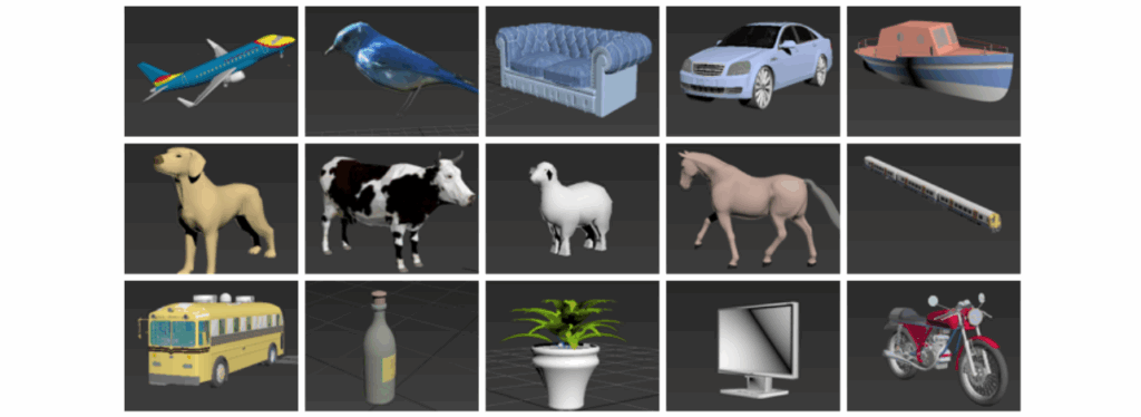
    Thus, the main question for Peng et al. was to separate different “visual cues”, i.e., different components of an object. Simplistic synthetic data does pretty well in terms of shape, but poorly in terms of texture or realistic varied poses, and the background will have to be inserted separately so it probably won’t match too well. Given this discrepancy in quality, what can we expect from object detection models?

    To study this question, Peng et al. propose an object detection pipeline that looks like R-CNN but is actually even simpler than that:

    They used AlexNet pretrained on ImageNet as a feature extractor, and trained classifiers on features extracted from region proposals, just like R-CNN. Then they started testing for robustness to various cues, producing different synthetic datasets and testing object detection performance on a real test set after training on these datasets. Here is a sample table of results from their paper.
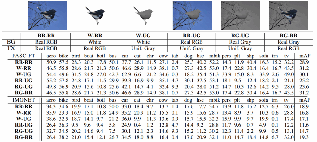
    What do we see in this table? Well, interestingly, the results do not follow the standard intuition that the more details you have, the better the results will be. The simplest synthetic data, the W-UG row with uniform gray objects on white backgrounds, yields very reasonable results and significantly outperforms gray objects on more complex backgrounds.

    On the other hand, experiments by Peng et al. show that adding a more varied set of views for a given object always helps, sometimes significantly. In the tables below, adding another view for synthetic shapes leads to improvements in the final quality on real test datasets.

    The absolute numbers in these tables did not really represent state of the art in object detection even in 2015, and are definitely not relevant today. But conclusions and comparisons show an important trend that goes through many early results on synthetic data for computer vision: for many models, the details and textures don’t matter as much since the models are looking for shapes and object boundaries. If that is the case for your model, then it is much more important to have a variety of shapes and poses, and textures can be left as an afterthought.

    By now, I would probably generalize this lesson: different cues may be of different importance to different models. So unless you are willing to invest some serious resources into making an effort to achieve photorealism across the board, experiment with your model and find out what aspects are really important and worth investing for, and what aspects can be neglected (e.g., in this case you can leave the objects gray and skip the textures). This is what Peng et al. teaches us, and I believe it is as relevant in 2020 as it was in 2015.

    First Attempts at Synthetic Videos for Object Detection

    This was the detailed part, and for a brief review today let us consider one of the first attempts to use synthetic videos for object detection by Bochinski et al. (2016), in a work called “Training a convolutional neural network for multi-class object detection using solely virtual world data“. This is one of the first attempts I could find at building a complete virtual world with the intent of making synthetic data for computer vision systems, and specifically for object detection.

    Bochinski et al. were also among the pioneers in using game engines for synthetic data generation. As the engine, they used Garry’s Mod, a sandbox game on the Source engine designed by Valve for Half Life and Counter Strike. Released in 2004 as a Half Life 2 mod intended to showcase the capabilities of the Source engine, Garry’s Mod remains a popular game even today; I saw it among my Steam recommendations less than a month ago…

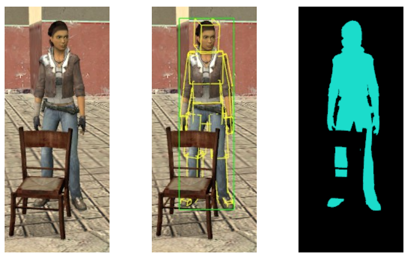
    Anyway, the point of both Garry’s Mod and its use in Bochinski et al. is that Source has a very capable physics engine, and even more than that, it supports scripting for bots, both human and vehicles. Thus, it is relatively easy to create a simulated world for urban driving applications, complete with humans, cars, and surveillance cameras placed in realistic positions. Bochinski et al. extended the engine to be able to export bounding boxes, segmentation, and other kinds of labeling:
    As for the rest, the Source engine allows to vary lighting conditions and, naturally, place cameras at arbitrary positions, e.g., in realistic surveillance camera locations:

    For object detection, since Bochinski et al. work with video data, they used a simple classical technique to construct bounding boxes: background subtraction. Basically, this means that they train a Gaussian mixture model to describe the history of every pixel, and if the pixel becomes different enough, it is considered to be part of the foreground (an object) rather than background. CNNs are only used (and trained) to do classification in the resulting bounding boxes. As a result, they achieve pretty good results even on a real test set:
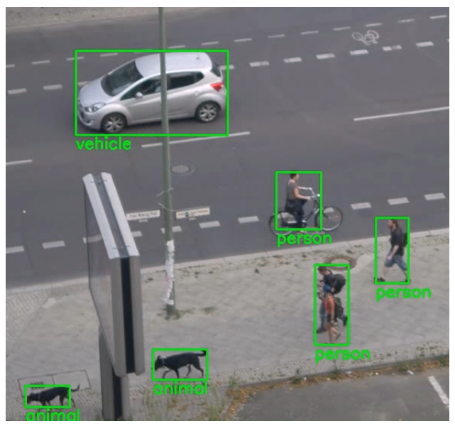
    So what’s the takeaway? This paper exemplifies how synthetic data can be helpful even for outdated pipelines: here, the bounding boxes were detected with a classical algorithm, so synthetic data was only used to train the classifier, and it still helped and resulted in a reasonable surveillance application.

    Conclusion

    Today, we have begun our account of synthetic data used to improve object detection pipelines. In fact, it is not easy to find papers that concentrate on object detection: since with synthetic data you can get any kind of labeling for free, most works skip right to segmentation or even more complex 3D-related problems. We have discussed two relatively early works (from 2015 and 2016) that, I believe, have something to tell us even today.

    The main takeaway point is, in my opinion, this: different models may prove to be robust to the (un)realism of different aspects of synthetic data. This means that in practice, when you develop a synthetic dataset for an existing model or class of models for a given problem, it often pays to produce an ablation study and find out where you need to invest the most effort. Next time, we will move on to multiple object detection in constrained spaces — stay tuned!

    Sergey Nikolenko
    Head of AI, Synthesis AI
  • Object Detection with Synthetic Data II: Common Objects And Their Context

    Object Detection with Synthetic Data II: Common Objects And Their Context

    In the last post, we started talking about object detection. We discussed what the problem is, saw the three main general-purpose real-world datasets for object detection, and began talking about synthetic data. Today, we continue the series with a brief overview of the most important synthetic datasets for object detection. Last time, I made an example of an autonomous driving dataset, but this is a topic of its own, and so are, say, synthetic images of people and human faces. Today, we will concentrate on general-purpose and household object datasets.

    ShapeNet, PartNet, and YCB: Common Objects in 3D

    The notion of synthetic data has been a staple of computer vision for a long time. Earlier on this blog, we talked about synthetic data in the very first computer vision models. But the first synthetic datasets all dealt with low-level computer vision problems such as, e.g., optical flow estimation, which are not our subject today. Large-scale public datasets for high-level computer vision problems with common everyday objects and scenes started to appear only in the mid-2010s.

    The first efforts related to recognizing everyday objects such as retail items, food, or furniture, mostly drew upon the same database for 3D models. Developed by Chang et al., ShapeNet indexes more than three million models, with 220000 of them classified into 3135 categories that match WordNet synsets. Apart from class labels, ShapeNet also includes geometric, functional, and physical annotations, including planes of symmetry, part hierarchies, weight and materials, and more. Researchers often used the clean and manually verified ShapeNetCore subset that covers 55 common object categories with about 51000 unique 3D models; see, e.g., a large-scale effort in 3D shape reconstruction by Yi et al. (2017).

    To be honest, ShapeNet looks more like 3D modeling from the 1990s than a five-year-old effort. Here are some sample shapes:

    But to some extent, this was intentional: works based on ShapeNet tried to prove that you can use even relatively crude models to teach neural networks to recognize objects. Rougher models are also easier to process. Since ShapeNet provides not only RGB images with ground truth bounding boxes and segmentation but also full 3D models, it has been widely used for projects on 3D shape reconstruction and completion and 3D scene understanding; maybe we will come back to these projects in a later post.

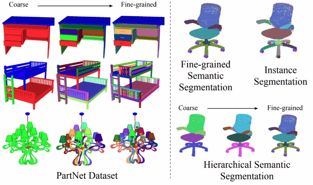
    This emphasis on 3D shape reconstruction carried over to one of the next iterations of ShapeNet, called PartNet (Mo et al., 2018). The creators of this dataset took ShapeNet models and provided an even more detailed kind of labeling for them. For instance, when you look at an office chair, you not only see a generic “chair” objects but can also distinguish the seat, back, armrests, and many other component parts of the chair. PartNet provides several layers of granularity for the parts of individual objects:

    They have done it on scale: according to Mo et al., PartNet contains 573,585 fine-grained annotations of object parts for 26,671 shapes that belong to 24 different object categories. The categories themselves are all common household objects but pretty diverse:

    To the best of our knowledge, PartNet remains the best dataset that you can use if you need a well-detailed chair with detailed parts annotation. It has been used in dozens of papers on object understanding, and the only thing that prevents it from having a wider impact on, say, indoor navigation is the relatively small selection of object categories. We hope that further efforts will be made to expand the diversity of object categories in PartNet or similar datasets.

    At about the same time, researchers from Yale, Carnegie Mellon, and Berkeley got together to produce another popular dataset of 3D shapes (Calli et al., 2015). True patriots of their respective alma maters, they named it the Yale-CMU-Berkeley (YCB) Object and Model set, and it was oriented towards applications in robotics. YCB collected not only the 3D shapes of objects but also their physical properties: dimension in real millimeters, mass, and frictional properties. The dataset was intended to help robotics researchers establish common benchmarks for object manipulation that could be used in silico, without expensive real experiments. Here is a sample of YCB data that would make Andy Warhol proud:

    To sum up, by now we have large-scale datasets of common objects in the form of 3D shapes. These datasets have hundreds of thousand shapes and can produce potentially infinite datasets. This does not, however, quite scale to the entire computer vision problem: even the largest existing datasets have quite restricted sets of object categories. We will see a wider variety in specific applications such as indoor or outdoor navigation.

    Now let’s see what we can do with those shapes!

    Flying Chairs and Falling Things: The Power of Domain Randomizations

    Once you have these basic objects, it’s time to put them into context. If you recall, last time we spoke about real-world object detection datasets, and I said (but not yet explained) that the problem becomes much harder if the same picture contains objects on different scales (small and large in terms of the proportion of the picture) and if the objects are embedded into a rich context (complex background). Naturally, if you have a synthetic chair centered on a white background, like in the images above, you won’t get a hard object detection problem, and a network trained on this kind of dataset won’t get you very far in real object detection.

    So what do we do? On the surface, it looks like we might have to bite the bullet and start developing complex backgrounds that capture realistic 3D scenes. People actually do it in, say, creating simulations and datasets for training self-driving cars, and it is an entirely reasonable investment of time and effort.

    But in object detection, sometimes even much simpler things can work well. Some of the hardest problems in object detection come from the complex interactions between objects: partial occlusions, different scales caused by different distances to the camera, and so on. So why don’t we use a more or less generic scene and just put the objects there at random, striving to achieve a cluttered and complicated scene but with little regard to physical plausibility?

    This plays into the narrative of domain randomization, a general term that means randomizing the parameters of synthetic scenes in order to capture as wide a variety of synthetic data as possible. The idea is that if the network learns to do its job on an extremely wide and varied distribution of data, it will hopefully do the job well on real data as well, even if individual samples of this synthetic data are very far from realistic. Starting from the paper by Tobin et al. (2017), domain randomization has been instrumental in synthetic data research, and we will definitely discuss it in more detail later.

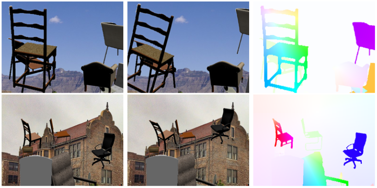
    When you put this idea into practice, you get datasets like Flying Chairs and Falling Things. Flying Chairs (Dosovitskiy et al., 2015) and Flying Chairs 3D (Mayer et al., 2015) were more oriented towards low-level problems such as optical flow estimation, so maybe I’ll talk about them in another post when it comes to that. The datasets look like this, by the way, so “flying chairs” is an apt name:

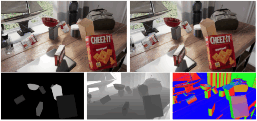
    The Falling Things Dataset (FAT), developed by NVIDIA researchers Tremblay et al. (2018), contains about 61500 images of 21 household objects taken from the YCB dataset and placed into virtual environments under a wide variety of lighting conditions, with 3D poses, pixel-perfect segmentation, depth images, and 2D/3D bounding box coordinates for each object. The virtual environments are realistic enough, but the scenes are purely random, with a lot of occlusions and objects just flying in the air in all directions. Here is a sample, complete with segmentation and depth maps:

    You can download the dataset by a link posted here; note that it is 42GB in size, although there are only 21 objects considered there. This is a common theme as well: as synthetic datasets grow in scale, it becomes less and less practical to render them in full glory and shoot the pictures back and forth over a network. Procedural generation is increasingly used to avoid this and render images only on a per-need basis.

    Synthetic Data For Your Project

    By this time, you probably wonder just how much effort has to go into creating a synthetic dataset of your own. If you need a truly large-scale dataset, it may be a lot, and so far there is no way to save on the actual design of 3D models. But, as it always happens in our industry, people are working hard to commoditize the things that all these projects have in common, in this case the randomization of scenes, object placement, lighting, and other parameters, as well as procedural generation of these randomized scenes.

    One recent example is NVIDIA’s Dataset Synthesizer (NDDS), a plugin for Unreal Engine 4 that allows computer vision researchers to easily turn 3D models and textures into prepared synthetic datasets. NDDS can produce RGB images, segmentation maps, depth maps and bounding boxes, and if the 3D models contain keypoints for the objects, then these keypoints and object poses can be exported too. What’s even more important, NDDS has automated tools for scene randomization: you can randomize lighting conditions, camera location, poses, textures, and more. Basically, NDDS makes it easy to create your own dataset similar to, say, Falling Things, and the result can look something like this:

    NVIDIA researchers are already using NDDS to produce synthetic datasets for computer vision; this is an important area of research for NVIDIA today. For example, SIDOD (Synthetic Image Dataset for 3D Object Pose Recognition with Distractors) by Jalal et al.; the image above is actually taken from their paper. SIDOD is relatively small by today’s standards, only 144K stereo image pairs, but it is one of the first datasets to combine all types of outputs with flying distractors. I will borrow a comparison table from the paper by Jalal et al. where you can see some of the datasets we discussed today:

    But even with this said, I still have to emphasize that for many real-life problems, you will definitely need professional help with the preparation of 3D models and construction of 3D scenes for them: even the power of domain randomization and random backgrounds could be much improved if you take pains to create a more proper context.

    Conclusion

    For the last two blog posts, we have been talking about object detection, but so far it has been purely from the point of view of the data. In the first post, we saw the object detection problem and real-world datasets for it, and today we have discussed some important synthetic datasets for this problem. But we are yet to talk about the actual solutions for object detection: okay, I got the data, but what do I actually do to solve the problem? Next time, I intend to start talking about just that.

    Sergey Nikolenko
    Head of AI, Synthesis AI

  • Object Detection with Synthetic Data I: Introduction to Object Detection

    Object Detection with Synthetic Data I: Introduction to Object Detection

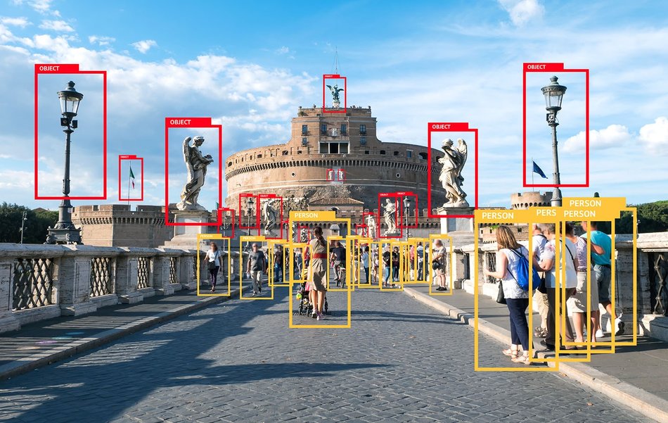
    Today, we begin a new mini-series that marks a slight change in the direction of the series. Previously, we have talked about the history of synthetic data (onetwothreefour) and reviewed a recent paper on synthetic data. This time, we begin a series devoted to a specific machine learning problem that is often supplemented by the use of synthetic data: object detection. In this first post of the series, we will discuss what the problem is and where the data for object detection comes from and how you can get your network to detect bounding boxes like below (image source).

    Problem Setting: What Is Object Detection

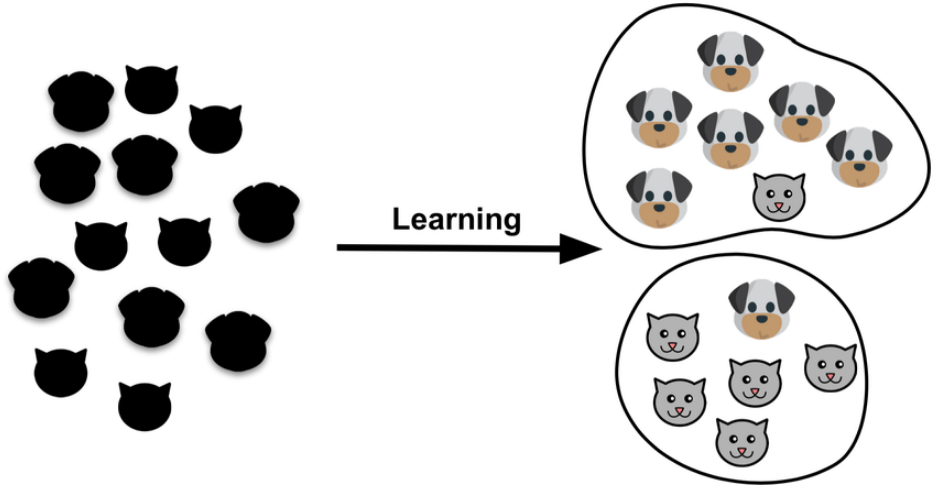
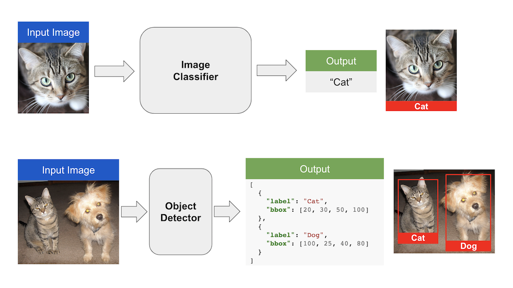
    If you have had any experience at all with computer vision, or have heard one of many introductory talks about the wonders of modern deep learning, you probably know about the image classification problem: how do you tell cats and dogs apart? Like this (image source):

    Even though this is just binary classification (a question with yes/no answers), this is already a very complex problem. Real world images “live” in a very high-dimensional space, on the order of millions of features: for example, mathematically a one-megapixel color photo is a vector of more than three million numbers! Therefore, the main focus of image classification lies not in the actual learning of a decision surface (that separates classes) but in feature extraction: how do we project this huge space onto something more manageable where a separating surface can be relatively simple?

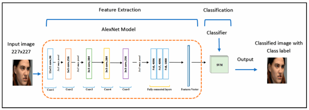
    This is exactly the reason why deep learning has taken off so well: it does not rely on handcrafted features like SIFT that people had used for computer vision before but rather learns its own features from scratch. The classifiers themselves are still really simple and classical: almost all deep neural networks for classification end with a softmax layer, i.e., basically logistic regression. The trick is how to transform the space of images to a representation where logistic regression is enough, and that’s exactly where the rest of the network comes in. If you look at some earlier works you can find examples where people learn to extract features with deep neural networks and then apply other classifiers, such as SVMs (image source):

    But by now this is a rarity: once we have enough data to train state of the art feature extractors, it’s much easier and quite sufficient to have a simple logistic regression at the end. And there are plenty of feature extractors for images that people have developed over the last decade: AlexNet, VGG, Inception, ResNet, DenseNet, EfficientNet…

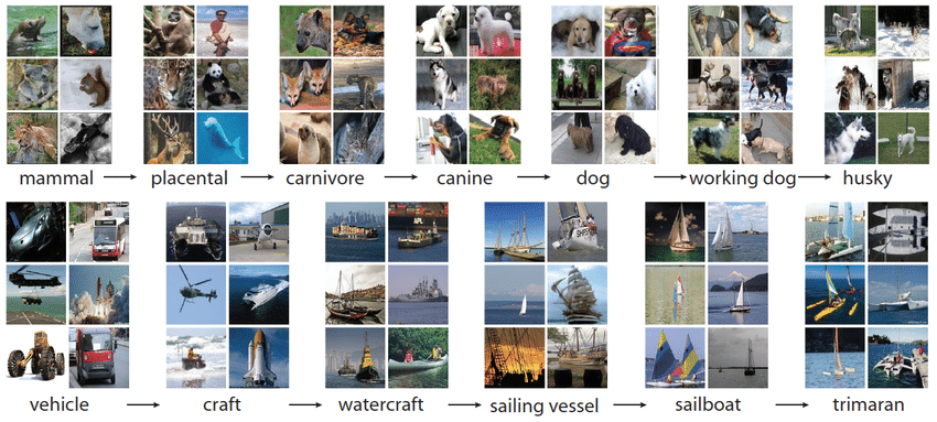
    It would take much more than a blog post to explain them all, but the common thread is that you have a feature extraction backbone followed by a simple classification layer, and you train the whole thing end to end on a large image classification dataset, usually ImageNet, a huge manually labeled and curated dataset with more than 14 million images labeled with nearly 22000 classes that are organized in a semantic hierarchy (image source):

    Once you are done, the network has learned to extract informative, useful features for real world photographic images, so even if your classes do not come from ImageNet it’s usually a matter of fine-tuning to adapt to this new information. You still need new data, of course, but usually not on the order of millions of images. Unless, of course, it’s a completely novel domain of images, such as X-rays or microscopy, where ImageNet won’t help as much. But we won’t go there today.

    But vision doesn’t quite work that way. When I look around, I don’t just see a single label in my mind. I distinguish a lot of different objects within my field of view: right now I’m seeing a keyboard, my own hands, a monitor, a coffee cup, a web camera and so on, and so forth, all basically at the same time (let’s not split hairs over the saccadic nature of human vision right now: I would be able to distinguish all of these objects from a single still image just as well).

    This means that we need to move on from classification, which assigns a single label to the whole image (you can assign several with multilabel classification models, but each of them will still refer to the entire image), to other problems that require more fine-grained analysis of the objects on images. People usually distinguish between several different problems:

    • classification, as we discussed above;
    • classification + localization, where you still assume there is only one “central” object on the image but you are also supposed to localize the object, that is, draw a bounding box (rectangle) around it;
    • object detection, our main topic today, requires to find multiple objects on the same picture, all with their own bounding boxes;
    • finally, segmentation is an even more complex problem: you are supposed to find the actual outlines of the objects, i.e., basically classify every pixel on the image into either one of the objects or the background; there are several different flavors to segmentation too (semantic, boundary, and instance segmentation) but that’s a discussion for another day.

    As explained with cats and dogs right here (image source):

    Mathematically, this means that the output of your network is no longer just a class label. It is now several (how many? that’s a very good question that we’ll have to answer somehow) different class labels, each with an associated rectangle. A rectangle is defined by four numbers (coordinates of two opposing corners, or one corner, width and height), so now each output is mathematically four numbers and a class label. Here is the difference (image source):

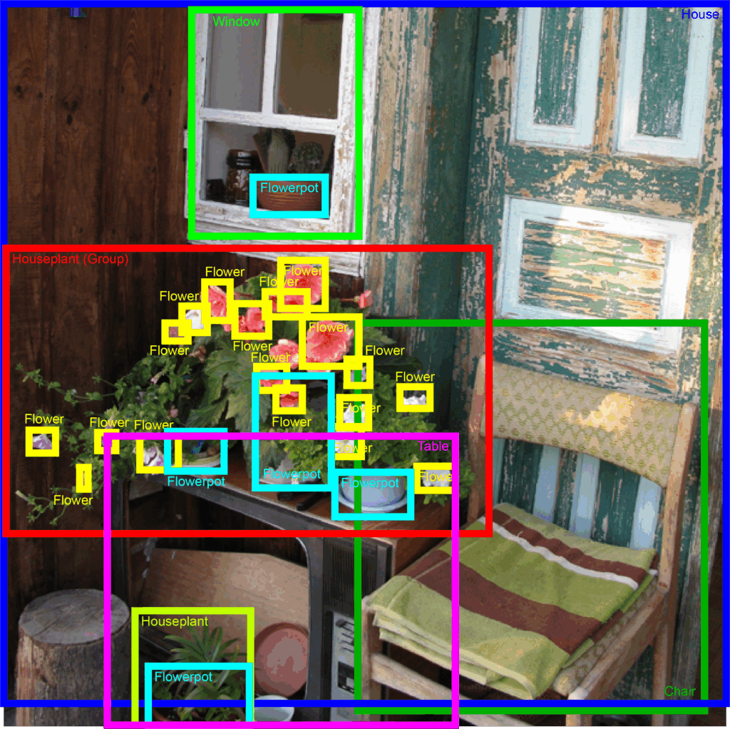
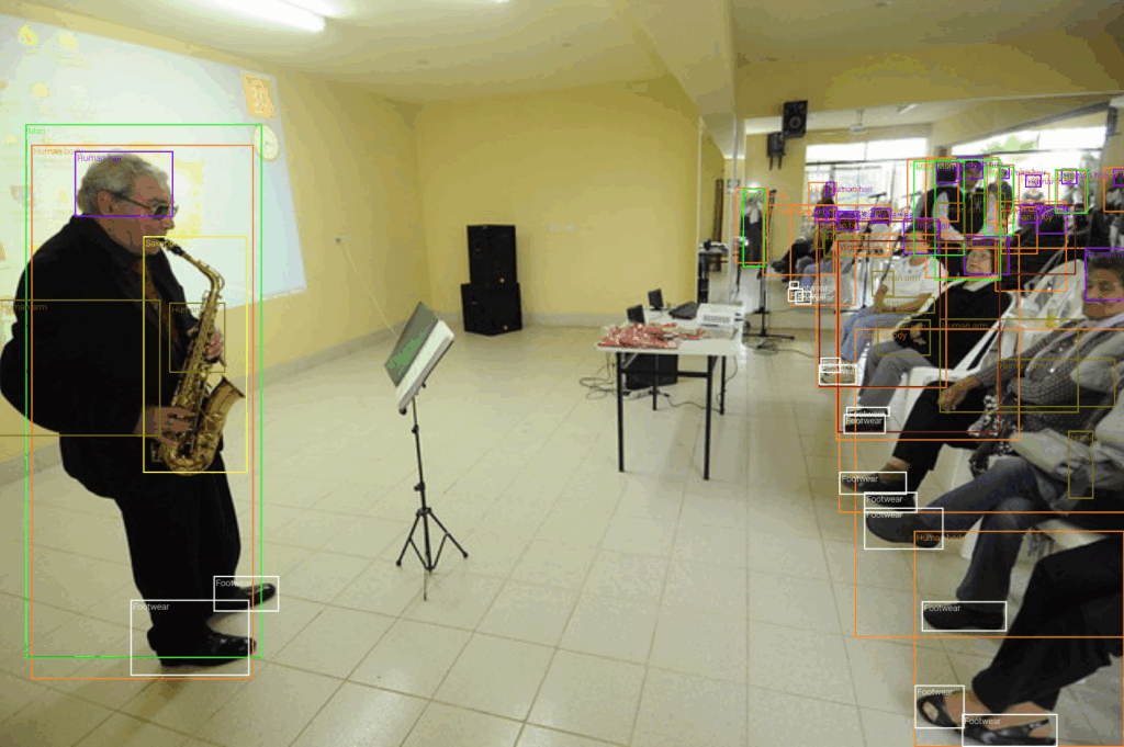
    From the machine learning perspective, before we even start thinking about how to solve the problem, we need to find the data. The basic ImageNet dataset will not help: it is a classification dataset, so it has labels like “Cat”, but it does not have bounding boxes! Manual labeling is now a much harder problem: instead of just clicking on the correct class label you have to actually provide a bounding box for every object, and there may be many objects on a single photo. Here is a sample annotation for a generic object detection problem (image source):

    You can imagine that annotating a single image by hand for object detection is a matter of whole minutes rather than seconds as it was for classification. So where can large datasets like this come from? Let’s find out.

    Object Detection Datasets: The Real

    Let’s first see what kind of object detection datasets we have with real objects and human annotators. To begin with, let’s quickly go over the most popular datasets, so popular that they are listed on the TensorFlow dataset page and have been used in thousands of projects.

    The ImageNet dataset gained popularity as a key part of the ImageNet Large Scale Visual Recognition Challenges (ILSVRC), a series of competitions held from 2010 to 2017. The ILSVRC series saw some of the most interesting advances in convolutional neural networks: AlexNet, VGG, GoogLeNet, ResNet, and other famous architectures all debuted there.

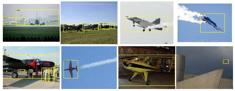
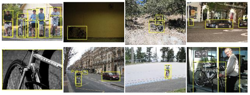
    A lesser known fact is that ILSVRC always had an object detection competition as well, and the ILSVRC series actually grew out of a collaborative effort with another famous competition, the PASCAL Visual Object Classes (VOC) Challenge held from 2005 to 2012. These challenges also featured object detection from the very beginning, and this is where the first famous dataset comes from, usually known as the PASCAL VOC dataset. Here are some sample images for the “aeroplanes” and “bicycle” categories (source):

    By today’s standards, PASCAL VOC is rather small: 20 classes and only 11530 images with 27450 object annotations, which means that PASCAL VOC has less than 2.5 objects per image. The objects are usually quite large and prominent on the photos, so PASCAL VOC is an “easy” dataset. Still, for a long time it was one of the largest manually annotated object detection datasets and was used by default in hundreds of papers on object detection.

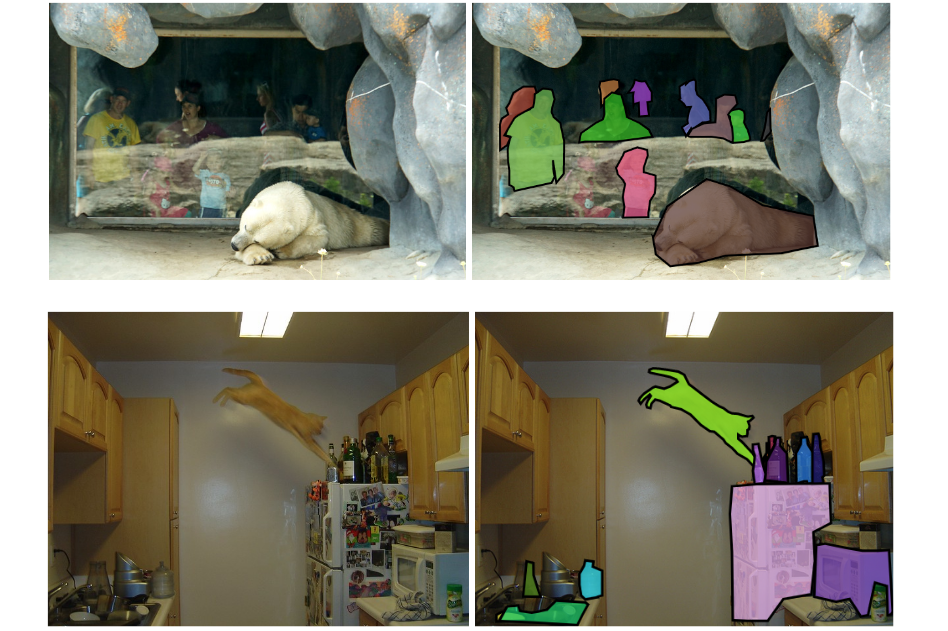
    The next step up in both scale and complexity was the Microsoft Common Objects in Context (Microsoft COCO) dataset. By now, it has more than 200K labeled images with 1.5 million object instances, and it provides not only bounding boxes but also (rather crude) outlines for segmentation. Here are a couple of sample images:

    As you can see, the objects are now more diverse, and they can have very different sizes. This is actually a big issue for object detection: it’s hard to make a single network detect both large and small objects well, and this is the major reason why MS COCO proved to be a much harder dataset than PASCAL VOC. The dataset is still very relevant, with competitions in object detection, instance segmentation, and other tracks held every year.

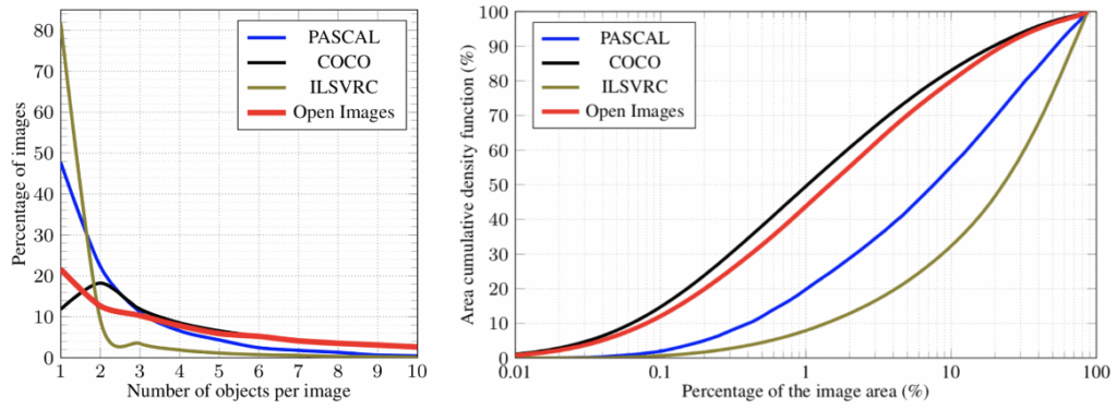
    The last general-purpose object detection dataset that I want to talk about is by far the largest available: Google’s Open Images Dataset. By now, they are at Open Images V6, and it has about 1.9 million images with 16 million bounding boxes for 600 object classes. This amounts to about 8.4 bounding boxes per image, so the scenes are quite complex, and the number of objects is also more evenly distributed:

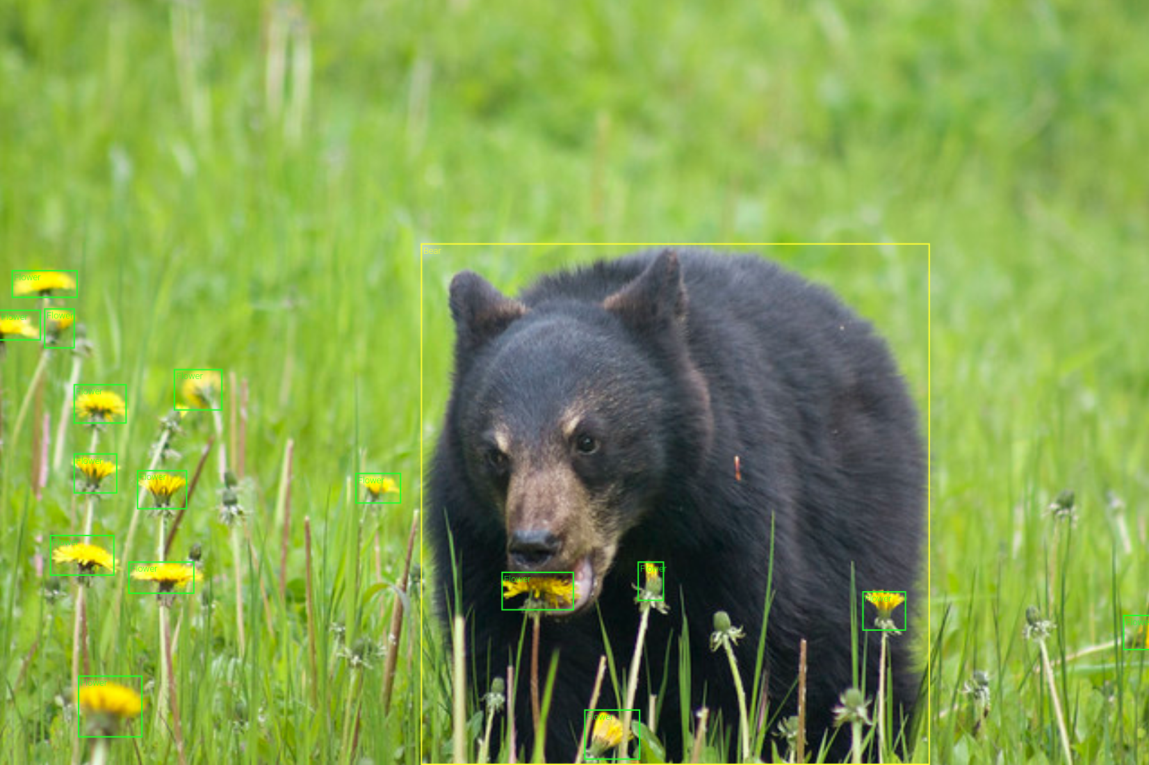
    Examples look interesting, diverse, and sometimes very complicated:

    Actually, Open Images was made possible by advances in object detection itself. As we discussed above, it is extremely time-consuming to draw bounding boxes by hand. Fortunately, at some point existing object detectors became so good that we could delegate the bounding boxes to machine learning models and use humans only to verify the results. That is, you can set the model to a relatively low sensitivity threshold, so that you won’t miss anything important, but the result will probably have a lot of false positives. Then you ask a human annotator to confirm the correct bounding boxes and reject false positives.

    As far as I know, this paradigm shift occurred in object detection around 2016, after a paper by Papadopoulos et al. It is much more manageable, and this is how Open Images became possible, but it is still a lot of work for human annotators, so only giants like Google can afford to put out an object detection dataset on this scale.

    There are, of course, many more object detection datasets, usually for more specialized applications: these three are the primary datasets that cover general-purpose object detection. But wait, this is a blog about synthetic data, and we haven’t yet said a word about it! Let’s fix that.

    Object Detection Datasets: Why Synthetic?

    With a dataset like Open Images, the main question becomes: why do we need synthetic data for object detection at all? It looks like Open Images is almost as large as ImageNet, and we haven’t heard much about synthetic data for image classification.

    For object detection, the answer lies in the details and specific use cases. Yes, Open Images is large, but it does not cover everything that you may need. A case in point: suppose you are building a computer vision system for a self-driving car. Sure, Open Images has the category “Car”, but you need much, much more details: different types of cars in different traffic situations, streetlights, various types of pedestrians, traffic signs and so on and so forth. If all you needed was an image classification problem, you would create your own dataset for the new classes with a few thousand images per class, label it manually for a few hundred dollars, and fine-tune the network for new classes. In object detection and especially segmentation, it doesn’t work quite as easily.

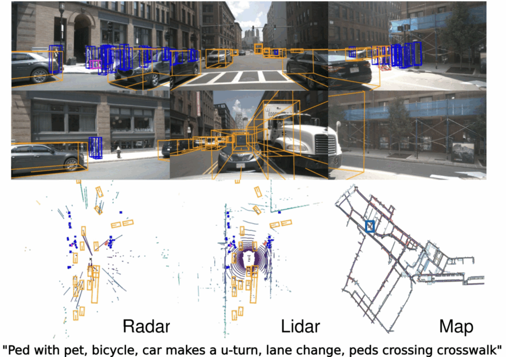
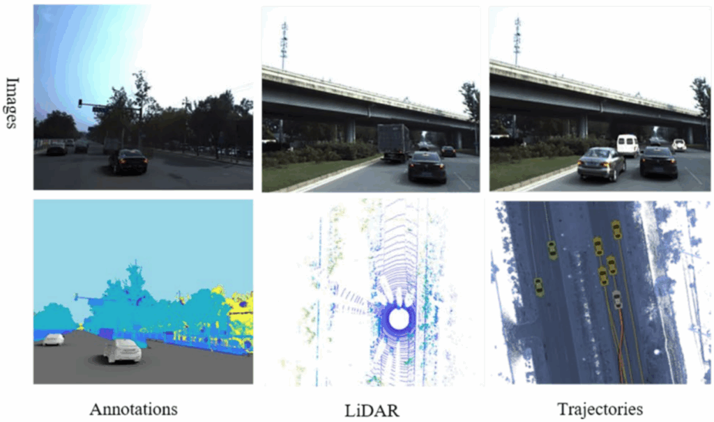
    Consider one of the latest and largest real datasets for autonomous driving: nuScenes by Caesar et al.; the paper, by the way, has been accepted for CVPR 2020. They create a full-scale dataset with 6 cameras, 5 radars, and a lidar, fully annotated with 3D bounding boxes (a new standard as we move towards 3D scene understanding) and human scene descriptions. Here is a sample of the data:

    And all this is done in video! So what’s the catch? Well, the nuScenes dataset contains 1000 scenes, each 20 seconds long with keyframes sampled at 2Hz, so about 40000 annotated images in total in groups of 40 that are very similar (come from the same scene). Labeling this kind of data was already a big and expensive undertaking.

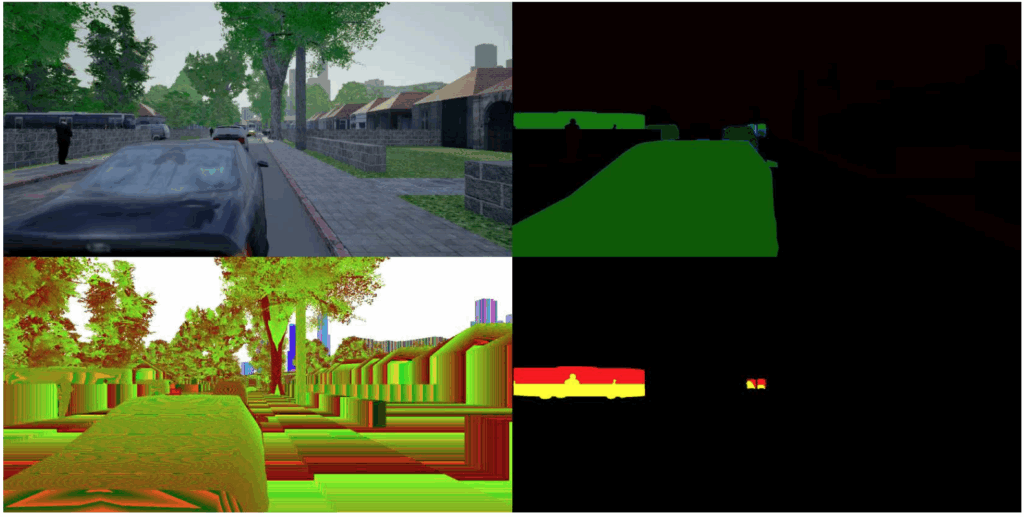
    Compare this with a synthetic dataset for autonomous driving called ProcSy. It features pixel-perfect segmentation (with synthetic data, there is no difference, you can ask for segmentation as easily as for bounding boxes) and depth maps for urban scenes with traffic constructed with the CityEngine by Esri and then rendered with Unreal Engine 4. It looks something like this (with segmentation, depth, and occlusion maps):

    In the paper, Khan et al. concentrate on comparing the performance of different segmentation models under inclement weather conditions and other factors that may complicate the problem. For this purpose, they only needed a small data sample of 11000 frames, and that’s what you can download from the website above (the compressed archives already take up to 30Gb, by the way). They report that this dataset was randomly sampled from 1.35 million available road scenes. But the most important part is that the dataset was generated procedurally, so in fact it is a potentially infinite stream of data where you can vary the maps, types of traffic, weather conditions, and more.

    This is the main draw of synthetic data: once you have made a single upfront investment into creating (or, better to say, finding and adapting) 3D models of your objects of interest, you are all set to have as much data as you can handle. And if you make an additional investment, you can even move on to full-scale interactive 3D worlds, but this is, again, a story for another day.

    Conclusion

    Today, we have discussed the basics of object detection. We have seen what kind of object detection datasets exist and how synthetic data can help with problems where humans have a really hard time labeling millions of images. Note that we haven’t said a single word about how to do object detection: we will come to this in later installments, and in the next one will review several interesting synthetic object detection datasets. Stay tuned!

    Sergey Nikolenko
    Head of AI, Synthesis AI
  • Synthetic Data Research Review: Context-Agnostic Cut-and-Paste

    Synthetic Data Research Review: Context-Agnostic Cut-and-Paste

    We have been talking about the history of synthetic data for quite some time, but it’s time to get back to 2020! I’m preparing a new series, but in the meantime, today we discuss a paper called “Learning From Context-Agnostic Synthetic Data” by MIT researchers Charles Jin and Martin Rinard, recently released on arXiv (it’s less than a month old). They present a new way to train on synthetic data based on few-shot learning, claiming to need very few synthetic examples; in essence, their paper extends the cut-n-paste approach to generating synthetic datasets. Let’s find out more and, pardon the pun, give their results some context.

    Problem Setting: Domain Shift and Context

    On this blog, there is no need to discuss in detail what synthetic data is all about; let me just link to my first post about the data problem in machine learning and to my recent survey of the field. Synthetic data is trying to solve this problem by presenting a potentially endless source of synthetic images after a one-time investment of resources to create the virtual objects/environments.

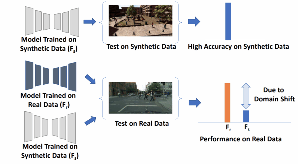
    However, this presents the obvious problem: you need to train on synthetic images but then apply the results on real photographs. This is an instance of the domain shift problem that sometimes appears in other fields as well (for instance, the “food” class looks very different in, say, the U.S. and Kenya). Here is an illustration of the domain shift problem for synthetic data from (Sankaranarayanan et al., 2018):

    Domain adaptation is a set of techniques designed to make a model trained on one domain of data, the source domain, work well on a different, target domain. This is a natural fit for synthetic data: in almost all applications, we would like to train the model in the source domain of synthetic data but then apply the results in the target domain of real data. By now, domain adaptation is a large field of machine learning, with many interesting models that either make input images more realistic (this is usually called refinement) or change the training process in such a way that the model does not differentiate between synthetic and real domains.

    We will definitely have many more posts that deal with domain adaptation in this blog. Today’s paper, however, is basically a modification of one of the most simple and straightforward approaches to generating synthetic datasets. Let us first discuss this idea in general and then get back to Jin and Rinard.

    Synthetic Objects Against Real Backgrounds

    Existing synthetic datasets also often exploit this idea of separating the object from the background. Usually it appears in the form of placing synthetic objects on real backgrounds. One usually has a virtually endless source of real backgrounds that are perfect for learning in every way but do not contain the necessary objects, so the idea is to paste synthetic objects in the most realistic way possible.

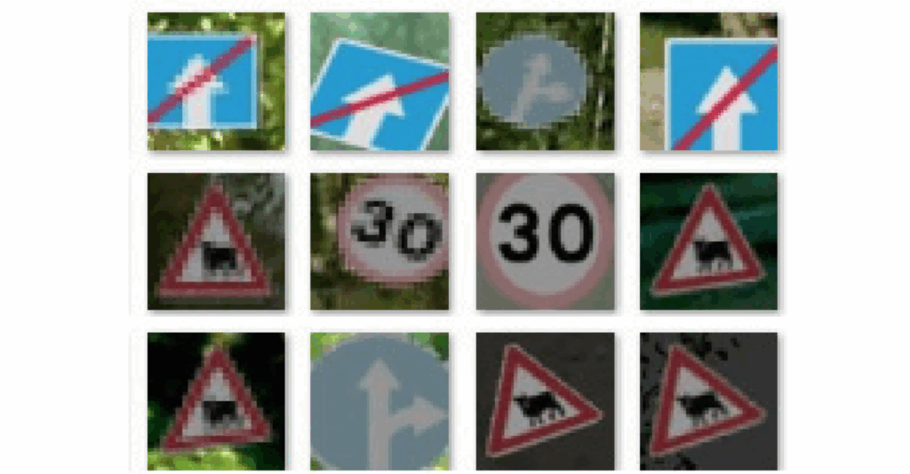
    In some problems, it is relatively straightforward. For example, one dataset mentioned in the paper by Jin and Rinard, SynSign by Moiseev et al. (2013), uses this trick to produce synthetic photographs of traffic signs. They cut out augmented (distorted) synthetic images of traffic signs and put them against real backgrounds:

    This is easy enough to do for traffic signs:

    • they are man-made objects with very simple textures, so even very simple synthetic images are pretty realistic;
    • they do not have to blend into the background because a traffic sign even on a real photo would be usually “hanging in the air” against a background that is some distance behind;
    • and most importantly, the resulting dataset’s resolution is quite small so you don’t have to worry about boundary artifacts.

    Modern synthetic data research can successfully apply the same trick to much more complex situations. For example, the Augmented Autonomous Driving Simulation (AADS) dataset (Li et al., 2019) helps train self-driving cars by blending synthetic cars against real-world backgrounds:

    I doubt you can even differentiate images in the top row from real photos of cars in context, especially given the relatively low resolution of this picture.

    AADS has a much more complex pipeline than just “cut-n-paste”, and I hope to talk to you about it in detail in a later post. But the basic point still stands: in many problems, 3D models of the objects of interest are far easier than 3D models of the entire environment, but at the same time there is a source of real-world backgrounds, and you can try to paste virtual objects onto them in a smart way to make realistic synthetic datasets.

    Balanced Sampling and Superimposing Objects

    Jin and Rinard take this approach to the next level. Basically, their paper still presents the same basic pipeline:

    • take the object space O consisting of synthetic objects placed in random poses and subjected to a number of different augmentations;
    • take the context space C consisting of background images;
    • superimpose objects from O against backgrounds from C at random;
    • train a neural network on the resulting composite images.

    The devil, however, is in the details; a few tricks take this simple approach to provide some of the very best results available in domain adaptation and few-shot learning.

    First, the sampling. One common pitfall of computer vision is that when you have relatively few examples of a class, they cannot come in a wide variety of backgrounds. Hence, in a process akin to overfitting the networks might start learning the characteristic features of the backgrounds rather than the objects in this class.

    What is the easiest way out of this? How can we tell the classifier that it’s the object that’s important and not the background? With synthetic images, it’s easy: let’s place several different objects on the same background! Then, since the labels are different, the classifier will be forced to learn that backgrounds are not important and it is the objects that differentiate between classes.

    Therefore, Jin and Rinard take care to introduce balanced sampling of objects and backgrounds. The basic procedure samples a random biregular graph so that every object is placed on an equal number of backgrounds and vice versa, every background is used with the same number of objects.

    But that’s not all. The second idea used in this paper stems from the obvious fact that the classifier must learn to distinguish between different objects. Therefore, it would be beneficial for training to concentrate on the hard cases where the classifier might confuse two objects.

    In the paper, this idea comes in two flavors. First, specifically for images Jin and Rinard suggest to superimpose one object on top of another, so that the previous object provides a maximally confusing context for the next one. A picture would be worth a thousand words here but, alas, the paper does not have any. But their second way to use the same idea is even more interesting.

    Robustness Training

    To give context to the idea of robustness training, I need to take a step back. You might remember how a few years ago, adversarial examples were all the rage. Remember this famous picture from Goodfellow et al. (2014)?

    What this means is that due to the simplified structure of neural networks (they are “too linear”, so to speak), you can find a direction in the image space such that even a small step in this direction (note the 0.007 coefficient in the linear combination) can lead to big changes in classifier predictions. How do we find this direction? Easy: just take a gradient of the loss function with respect to the input (rather than the weights, as in training) and go either where the correct class’ probability is reduced the most or where the probability of the class you want to get is increased the most. This is actually explained below the picture.

    Since 2013-2014, when adversarial examples first appeared, this field has come a long way. By now, there are a lot of different sorts of adversarial attacks, including attacks that work in the physical world (Kurakin et al., 2016): you can print out an adversarial image, take a photo, and it is still misclassified! The attacks also cause defenses to appear; naturally, attacks have the first move but usually you can defend against a given attack. A recent survey by Xu et al. (2019) lists about 150 references, and the field is growing.

    One of the easiest ways to defend against the attack above is to introduce changes into the training process. These gradients with respect to the input can be computed during training as well, so during training you can have access to adversarial examples. Hence, you can

    • either add extra components to the loss function, so that the classifier is penalized if it makes mistakes on the hardest examples in some neighborhood of the original image,
    • or simply add adversarial examples to the mix as a possible augmentation (this can be made basically equivalent to changing the loss function if you add them in the same mini-batch).

    This is exactly the idea of robustness training that Jin and Rinard suggest for synthetic images. You have a synthetic image that might look a little unrealistic and might not be hard enough to confuse even an imperfect classifier. What do you do? You can try to make it harder for the classifier by turning it into an adversarial example.

    With all these ideas combined, Jin and Rinard obtain a relatively simple pipeline that is able to achieve state-of-the-art results by training with only a single synthetic image of each object class. Note that there is no fancy domain adaptation here: all ideas can be thought of as smart augmentations.

    Conclusion

    Today, after a few posts on the history of synthetic data we are taking a break from long series. Here I have reviewed a recent paper from arXiv and discussed its ideas. This paper touches on many different ideas from different parts of machine learning. As we review additional papers in this series, we hope to highlight interesting research and add some new ideas of our own to the mix.

    Next time, we will have some more ideas to discuss. Until then!

    Sergey Nikolenko
    Head of AI, Synthesis AI

  • Synthetic Data for Early Robots, Part II: MOBOT and the Problems of Simulation

    Synthetic Data for Early Robots, Part II: MOBOT and the Problems of Simulation

    Last time, we talked about robotic simulations in general: what they are and why they are inevitable for robotics based on machine learning. We even touched upon some of the more philosophical implications of simulations in robotics, discussing early concerns on whether simulations are indeed useful or may become a dead end for the field. Today, we will see the next steps of robotic simulations, showing how they progressed after the last post with the example of MOBOT, a project developed in the first half of the 1990s in the University of Kaiserslautern. This is another relatively long read and the last post in the “History of Synthetic Data” series.

    The MOBOT Project

    Let’s begin with a few words about the project itself. MOBOT (Mobile Robot, and that’s the most straightforward acronym you will see in this post) was a project about a robot navigating indoor environments. In what follows, all figures are taken from the papers about the MOBOT project, so let me just list all the references up front and be done with them: (Buchberger et al., 1994), (Trieb, von Puttkamer, 1994), (Edlinger, von Puttkamer, 1994), (Zimmer, von Puttkamer, 1994), (Jorg et al., 1993), (Hoppen et al., 1990).

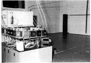
    Here is what MOBOT-IV looked like:

    Note the black boxes that form a 360 degree belt around the robot: these are sonar sensors, and we will come back to them later. The main problem that MOBOT developers were solving was navigation in the environment, that is, constructing the map of the environment and understanding how to go where the robot needed to go. There was this nice hierarchy of abstraction layers that gradually grounded the decisions down to the most minute details:

    And there were three different layers of world modeling, too; the MOBOT viewed the world differently depending on the level of abstraction:

    But in essence, this came down to the same old problem: figure out the sensor readings and map them to all these nice abstract layers where the robot could run pathfinding algorithms such as the evergreen A*. Apart from the sonars, the robot also had a laser radar, and the overall scheme of the ps-WM (Pilot Specific World Modeling; I told you the acronyms would only get weirder) project looks quite involved:

    Note that there are several different kinds of maps that need updating. But as we are mostly interested in how synthetic environments were used in the MOBOT project, let us not dwell on the detail and proceed to the simulation.

    The 3d7 Simulation Environment: Perfecting the Imperfections

    One of the earliest examples of a full-scale 3D simulation environments for robotics is the 3d7 Simulation Environment (Trieb, Puttkamer, 1994); the obscure name does not refer to a nonexistent seven-sided die but rather represents an acronym for “3D Simulation Environment”. The 3d7 environment was developed for MOBOT-IV, an autonomous mobile robot that was supposed to navigate indoor environments; it had general-purpose ambitions rather than simply being, say, a robot vacuum cleaner, because its scene understanding was inherently three-dimensional, while for many specific tasks a 2D floor map would be just enough.

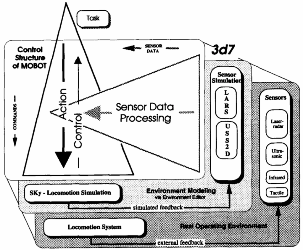
    The overall structure of 3d7 is shown on the figure below:

    It is pretty straightforward: the software simulates a 3D environment, robot sensors, and robot locomotion, which lets the developers to model various situations, choose the best algorithms for sensory data processing and action control, and so on, just like we discussed last time.

    The main point I wanted to make with this example is this: making realistic simulations is very hard. Usually, when we talk about synthetic data, we are concentrating on computer vision, and we are emphasizing the work it takes to create a realistic 3D environment. It is indeed a lot, but just creating a realistic 3D scene it’s definitely not the end of the story for robotics.

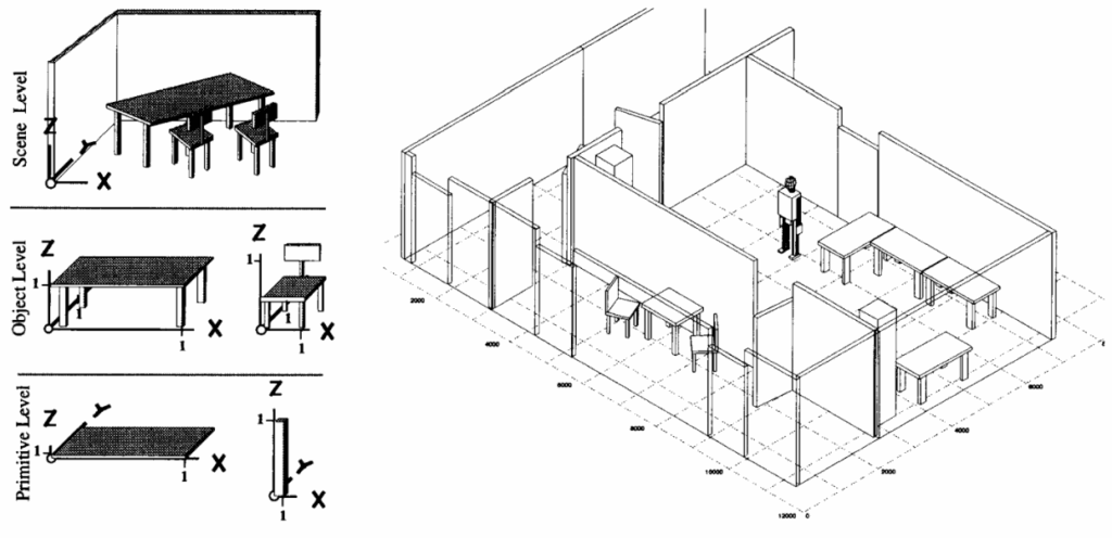
    3d7 contained an environment editor that let you place primitive 3D objects such as cubes, spheres, or cylinders, and also more complex objects such as chairs or tables. It produced a scene complete with the labels of semantic objects and geometric primitives that make up these objects, like this:

    But then the fun part began. MOBOT-IV contained two optical devices: a laser radar sensor and a brand new addition compared to MOBOT-III, an infrared range scanning device. This means that in order to make a useful simulation, the 3d7 environment had to simulate these two devices.

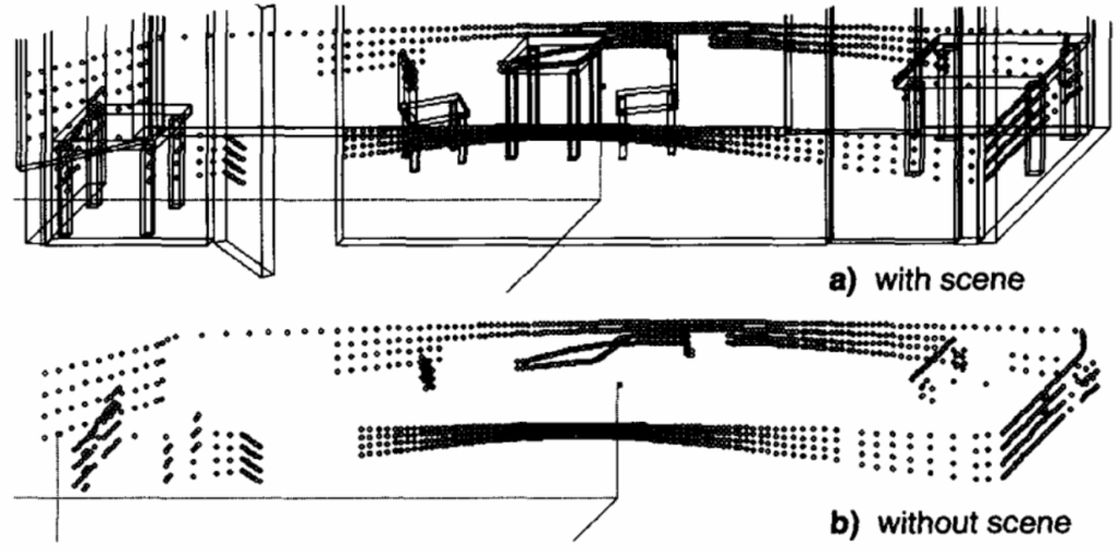
    It turns out that both these simulations represent interesting projects. LARS, the Laser Radar Simulator, was designed to model the real laser radar sensor of MOBOT-III and the new infrared range scanner of MOBOT-IV. It produced something like this:

    As for sonar range sensors, the corresponding USS2D simulator (Ultrasonic Sensor Simulation 2D) was even more interesting. It was based on the work (Kuc, Siegel, 1987) that takes about thirty pages of in-depth acoustic modeling. I will not go into the details but trust me, there are a lot of details there. The end result was a set of sonar range readings corresponding to the reflections from nearest walls:

    This is a common theme in early research on synthetic data, one we have already seen in the context of ALVINN. While modern synthetic simulation environments strive for realism (we will see examples later in the blog), early simulations did not have to be as realistic as possible but rather had to emulate the imperfections of the sensors available at the time. They could not simply assume that hardware is pretty good, they knew it wasn’t and had to incorporate models of their hardware as well.

    As another early example, I can refer to the paper (Raczkowsky, Mittenbuehler, 1989) that discussed camera simulations in robotics. It is mostly devoted to the construction of a 3D scene, and back in 1989, you had to do it all yourself, so the paper covers:

    • surfaces, contours, and vertices that define a 3D object;
    • optical surface properties including Fresnel reflection, diffuse reflectance, flux density and more;
    • light source models complete with radiance, wavelengths and so on;
    • and finally the camera model that simulates a lens system and the electronic hardware of the robot’s camera.

    In the 1980s, only after working through all that you could produce such marvelous realistic images as this 200×200 synthetic photo of some kind of workpieces:

    Fortunately, by now most of this is already being taken care of by modern 3D modeling software or gaming engines! However, camera models are still relevant in modern synthetic data applications. For instance, an important use case for, e.g., a smartphone manufacturer might be to re-train or transfer its computer vision models when the camera changes, and you need a good model for both the old and new cameras in order to capture this change and perform this transition.

    But wait, that’s not all! After all of this is done, you only have simulated the sensor readings! To actually test your algorithm you also need to model the actions your robot can take and how the environment will respond to these actions. In case of 3d7, this means a separate locomotion simulation model for robot movement called SKy (Simulation of Kinematics and Dynamics of wheeled mobile robots), which also merited its own paper but which we definitely will not go into. We will probably return to this topic in the context of more modern robotic simulations: this is a field that still needs to be done separately and cannot be lifted from gaming engines.

    Learning in MOBOT: Synthetic Data Strikes Again

    The MOBOT project did not contain many machine learning models, it was mostly operated by fixed algorithms designed to work with sensor readings as shown above. Even the 3d7 simulation environment was mostly designed to help test various data processing algorithms (world modeling) and control algorithms (e.g., path planning or collision avoidance), a synthetic data application similar to the early computer vision we talked about before.

    But at some point, MOBOT designers did try out some machine learning. The work (Zimmer, von Puttkamer, 1994) has the appetizing title Realtime-learning on an Autonomous Mobile Robot with Neural Networks. There are not, however, neural networks that you are probably used to: in fact, Zimmer and von Puttkamer used self-organizing maps (SOM), sometimes called Kohonen maps in honor of their creator (Kohonen, 1982), to cluster sensor readings.

    The problem setting is this: as the robot moves around its surroundings, it collects sensor information. The basic problem is to build a topological map of the floor with all the obstacles. To do that, the robot needs to be able to recognize places where it has already been, i.e., to cluster the entire set of sensor readings into “places” that can serve as nodes for the topological representation.

    Due to the imprecise nature of robotic movements we cannot rely on the kinematic model of where we tried to go: small errors tend to accumulate. Instead, the authors propose to cluster the sensor readings: if the current vector of readings is similar to what we have already seen before, we are probably in approximately the same place.

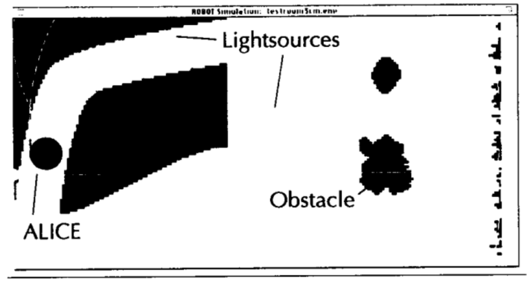
    And again we see the exact same effect: while Zimmer and von Puttkamer do present experiments with a real robot, most of the experiments for SOM training was done with synthetic data. It was done in a test environment that looks like this:

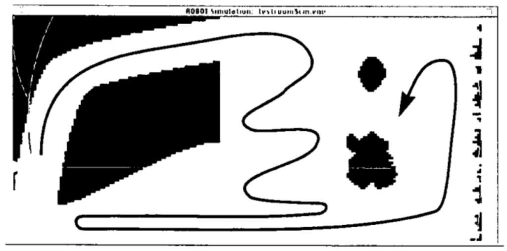
    with a test trajectory of the form

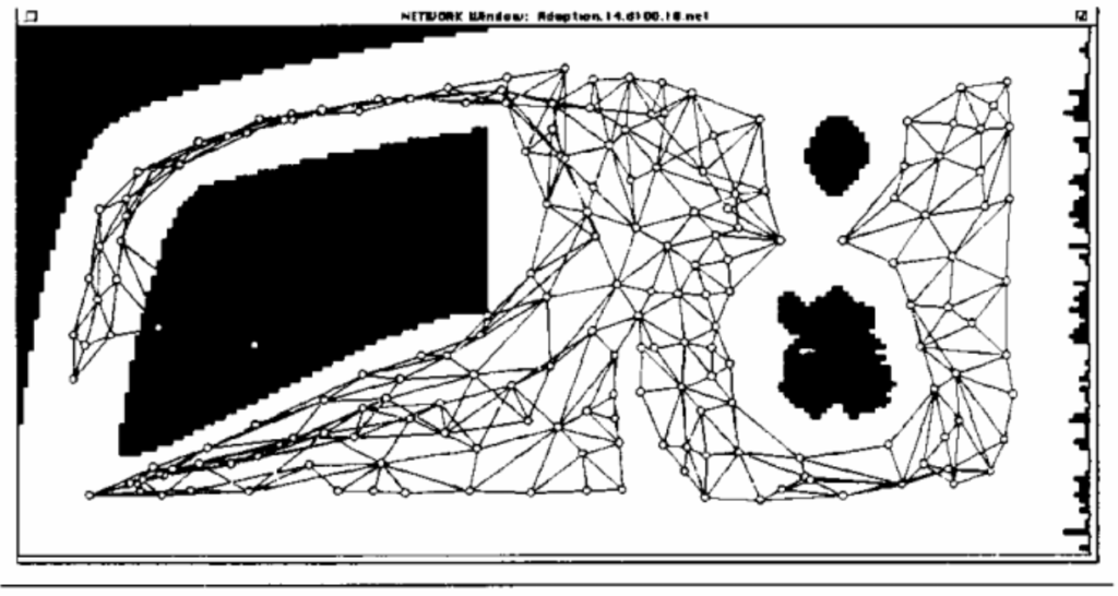
    And indeed, when the virtual robot has covered this trajectory, SOMs clustered nicely and allowed to build a graph, a topological representation of the territory:

    Conclusion

    Today, we have seen the main components of a robotic simulation system; we have discussed the many different aspects that need to be simulated and shown how this all came together in one early robotic project, the MOBOT from the University of Kaiserslautern.

    This post concludes the series devoted to the earliest applications of synthetic data. We talked about line drawings and test sets in early computer vision, the first self-driving cars, and spent two posts talking about simulations in robotics. All through the last posts, we have seen a common theme: synthetic data may not be necessary for classical computer vision algorithms. But as soon as any kind of learning appears in computer vision, synthetic data is not far behind. Even in the early days, it was used to test CV algorithms, to train models for something as hard as learning to drive or simply for clustering sensor readings to get a feeling for where you have been.

    I hope I have convinced you that synthetic data has gone hand in hand with machine learning for a long time, especially with neural networks. In the next posts, I will jump back to something on the bleeding edge of synthetic data research. Stay tuned!

    Sergey Nikolenko
    Head of AI, Synthesis AI

  • Synthetic Data for Robots, Part I: Are Simulations Good For Robotics?

    Synthetic Data for Robots, Part I: Are Simulations Good For Robotics?

    In the previous two blog posts, we have discussed the origins and first applications of synthetic data. The first part showed how early computer vision used simple line drawings for scene understanding algorithms and how synthetic datasets were necessary as test sets to compare different computer vision algorithms. In the second part, we saw how self-driving cars were made in the 1980s and how the very first application of machine learning in computer vision for autonomous vehicles, the ALVINN system, was trained on synthetic data. Today, we begin the discussion of early robotics and the corresponding synthetic simulators… but this first part will be a bit more philosophical than usual.

    Why Robots Need Simulators

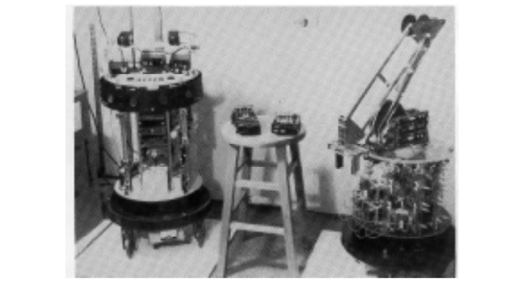
    Robotics is not quite as old as artificial intelligence: the challenge of building an actual physical entity that could operate in the real world was too big a hurdle for the first few years of AI. However, robotics was recognized as one of the major problems in AI very early on, and as soon as it became possible people started to build real world robots. Here is one of the earliest attempts at a robot equipped with a vision system, the Stanford Cart built in the 1970s (pictures taken from a later review paper by Hans Moravec):

    The Cart had an onboard TV system, and a computer program tried to drive the Cart through obstacle courses based on the images broadcast by this system. Based on several images taken from different camera positions (a kind of “super-stereo” vision), its vision algorithm tried to find interest points (features), detect obstacles and avoid or go around them. It was extremely successful for such an early system, although the performance was less than stellar: the Cart moved in short lurches, about 1 meter, every 10-15 minutes. Still, in these lurches the Cart could successfully avoid real life obstacles.

    As we discussed last time, before the 1990s computer vision was very seldom based on learning of any kind: researchers tried to devise algorithms, and data was only needed to test and compare them. This fully goes for robotics: early robots such as the Cart had hardcoded algorithms for vision, pathfinding, and everything else.

    However, experiments with the Cart and similar robots taught researchers that it is far too costly and often plain impossible to validate their ideas in the real world. Most researchers decided that they want to first test the algorithms in computer simulations and only then proceed to the real world. There are two main reasons for this:

    • it is, of course, far easier, faster, and cheaper to test new algorithms in a simulated world than embed them into real robots and test in reality;
    • simulations can abstract away many problems that a real world robot has to face, such as unpredictable sources of noise in sensor readings, imperfections in the hardware, accumulating errors and so on; it is important to be able to distinguish whether your algorithm does not work because it is a bad idea in general or because the sensor noise is too large in this particular case.

    Hence, robotics moved to the «simulate first, build second» principle which it abides to this day.

    A Sample Early Simulator

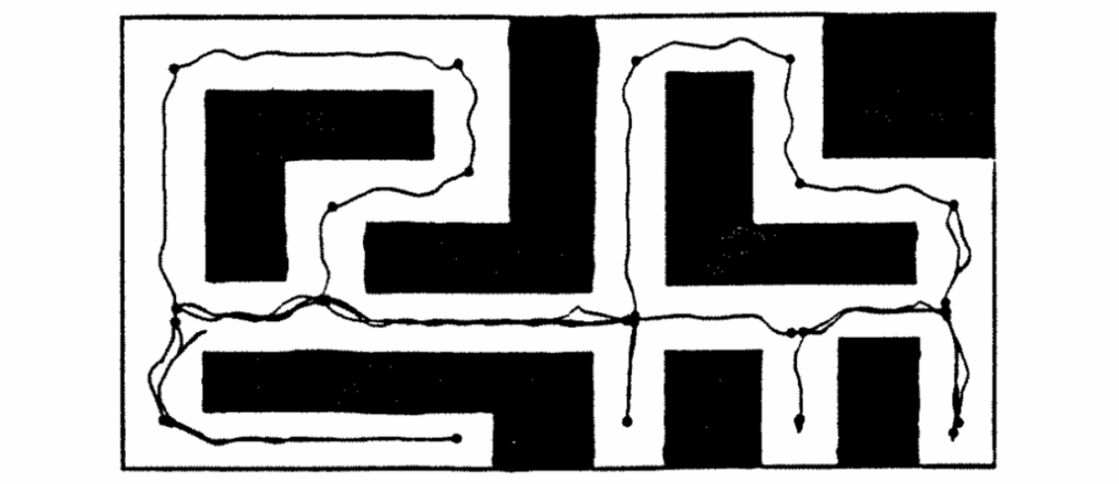
    Let’s have a look at a sample early simulator for a rover robot that was supposed to map the space around it. Benjamin Kuipers and Yung-Tai Byun developed an approach to robot exploration and mapping based on a semantic hierarchy of spatial representations (Kuipers and Byun, 1988; 1991). This means that their robot is supposed to gradually work its way up from the control level, where it finds distinctive places and paths, through the topological level, where it creates a topological network description of the environment, and finally to the geometric level, where the topology is converted to a geometric map by incorporating local information about the distances and global metric relationships between the places. The exploration paths could look something like this (all pictures taken from the AAAI paper):

    The method itself was a seminal work, but it’s not our subject right now and I will not go into any more details about it. But note their approach to implementing and testing the method: Kuipers and Byun programmed (in Common Lisp, by the way) a two-dimensional simulated environment called the NX Robot Simulator. The virtual robot in this environment has access to sixteen sonar-type distance sensors and a compass, and moves by two tractor-type chains. The interesting part of this simulation is that Kuipers and Byun took special care to implement error models for the sonars that actually reflect real life errors.

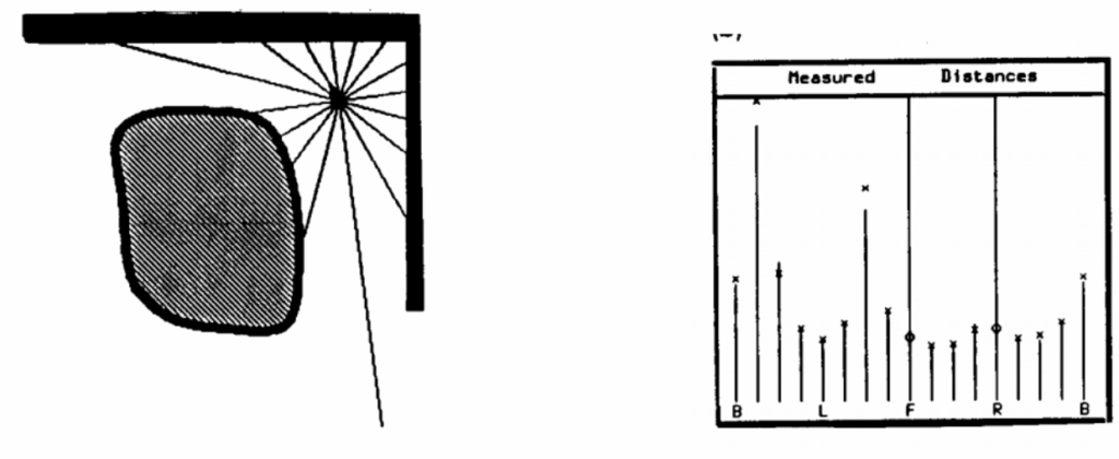
    Here is a sample picture from their simulation; on the left you see a robot shooting sonar rays in 16 directions, and the histogram on the right shows the sensor readings (with vertical lines) and true distances (with X and O markers). Note how the O markers represent a systematic error due to specular reflection, much more serious than the deviations of X markers that comes from normal random error:

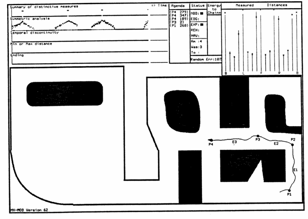
    They made it into a software product with a GUI interface, which was much harder to do in the 1980s than it is now. Here is a sample screenshot:

    The algorithms worked fine in a simulation, and the simulation was so realistic that it actually allowed to transfer the results to the real world. In a later work, Kuipers et al. (1993) report on their experiments with two physical mobile robots, Spot and Rover, that quite successfully implemented their algorithms on two different sensorimotor systems.

    Deep Criticisms: Simulations, Embodiment, and Representation

    Despite these successes, not everybody believed in computer simulations for robotics. In the same book as (Kuipers et al., 1993), another chapter by Rodney Brooks and Maja Mataric, aptly titled Real Robots, Real Learning Problems, had an entire section devoted to warning researchers in robotics from relying on simulations too much. Brooks and Mataric put it as follows:

    Simulations are doomed to succeed. Even despite best intentions there is a temptation to fix problems by tweaking the details of a simulation rather than the control program or the learning algorithm. Another common pitfall is the use of global information that could not possibly be available to a real robot. Further, it is often difficult to separate the issues which are intrinsic to the simulation environment from those which are based in the actual learning problem.

    Basically, they warned that computer vision had not been solved yet, and while a simulation might provide the robot with information such as «there is food ahead», in reality such high-level information would never be available. This, of course, remains true to this day, and modern robotic vision systems make use of all modern advances in object detection, segmentation, and other high-level computer vision tasks (where synthetic data also helps a lot, by the way, but this will be the subject of later posts).

    All this looks like some very basic points that are undoubtedly true, and they sound more as a part of the problem setting than true criticism. However, Rodney Brooks also presents a much more interesting criticism which is not so much against synthetic data and simulations as against the entire computer vision program for robotics; while this is an aside for this blog series, this is an interesting aside, and I want to elaborate on it.

    I will present Brooks’ ideas based on two of his papers, Intelligence Without Representation and Intelligence Without Reason. In the former, Brooks argues that abstract representation of the real world, which was a key feature of contemporary AI solutions, is a dangerous weapon that can lead to self-delusion. He says that real life intelligence has not evolved as a machine for solving well-defined abstract problems such as chess playing or theorem proving: intelligence in animals and humans is inseparable from perception and mobility. This was mostly a criticism of early approaches to AI that indeed concentrated on abstractions such as block worlds or knowledge engineering.

    In Intelligence Without Reason, Brooks goes further to argue that abstraction and knowledge are basically unavailable to systems that have to operate in the real world, that is, to robotic systems. For example, he mentions vision algorithms based on line drawings that we discussed a couple of blog posts ago, and admits that although some early successes in line detection had dated back to the 1960s, even in the early 1990s we did not have a reliable way to convert real life images to line drawings. «Try it! You’ll be amazed at how bad it is,» Brooks comments, and this comment is not so far from the truth even today.

    Brooks presents four key ideas that he believes to be crucial for AI:

    • situatedness, i.e., placing AI agents in the real world «with continuity, surprises, or ongoing history»; Brooks agrees that such a world would be hard to achieve in a simulation and concludes that «the world is its own best model»;
    • embodiment, i.e., physical grounding of a robot in the real world; this is important precisely to avoid the self-delusion pitfalls that inevitably abstract simulations may lead to; apart from new problems, embodiment may also present solutions to abstract problems by grounding the reasoning and conclusion in the real world;
    • intelligence, which Brooks proposes to model after simpler animals than humans, concentrating at first on perception and mobility and only then moving to abstract problem solving, like we did in the process of evolution;
    • emergence, where Brooks makes the distinction between traditional AI systems whose components are functional (e.g., a vision system, a pathfinding system, and so on) and behaviour-based systems where each functional unit is responsible for end-to-end processing needed to form a given behaviour (e.g., obstacle avoidance, gaze control etc.).

    As for simulations, Brooks concludes that they are examples of precisely the kind of abstractions that may lead to overly optimistic interpretations of results, and argues for complete integrated intelligent mobile robots.

    Interestingly, this resonates with the words of Hans Moravec that he wrote in his 1990 paper about the Stanford Cart robot that I began with:

    My conclusion is that solving the day to day problems of developing a mobile organism steers one in the direction of general intelligence, while working on the problems of a fixed entity is more likely to result in very specialized solutions

    Brooks put his ideas in practice, leading a long-term effort to create mobile autonomous robots in the MIT AI lab. Here are Allen, Herbert, Tom, and Jerry that were designed to interact with the world rather than plan and carry out plans:

    This work soon ran into technological obstacles: the hardware was just not up to the task in the late 1980s. But Brooks’ ideas live on: Intelligence Without Representation has more than 2000 citations and is still being cited in 2020, in fields ranging from robotics to cognitive sciences, nanotechnology, and even law (AI-related legislature is a hot topic, and I may return to it on this blog someday).

    Conclusion

    So are simulations useful for robotics? Of course, and increasingly so! While I believe that there is a lot of truth to the criticism shown in the previous section, in my opinion in most applications it boils down to the following: when your robot works in a simulation, it does not yet mean that it will work in real life. This is, of course, true.

    On the other hand, if your robot does not work even in a simulation, it is definitely too early to start building real systems. Moreover, modern developments in robotics such as the success of reinforcement learning seem to have a strange relationship with Brooks’ ideas. On the one hand, this is definitely a step in the direction of creating end-to-end systems that are behaviour-oriented rather than composed of clear-cut predesigned functional units. On the other hand, in the modern state of reinforcement learning it is entirely hopeless to suggest that systems could be trained in real life: they absolutely need simulations because they require millions of training episodes.

    In the next posts, we will consider other early robotic simulations and how their ideas still live on in modern synthetic environments for robotics.

    Sergey Nikolenko
    Head of AI, Synthesis AI
  • Synthetic Data: The Early Days, Part II

    Synthetic Data: The Early Days, Part II

    We continue from last time, when we began a discussion of the origins and first applications of synthetic data: using simple artificial drawings for specific problems and using synthetically generated datasets to compare different computer vision algorithms. Today, we will learn how people made self-driving cars in the 1980s and see that as soon as computer vision started tackling real world problems with machine learning, it could not avoid synthetic data.

    Early self-driving cars: from Futurama to Alvin

    Self-driving cars are hot. By now, self-driving trucks and buses certified for closed environments such as production facilities or airports are already on the market, and many different companies are working towards putting self-driving passenger cars on the roads of our cities. This kind of progress always takes longer than expected, but by now I believe that we are truly on the verge of a breakthrough (or maybe the breakthrough has already happened and will soon appear on the market). In this post, however, I want to turn back to the history of the subject.

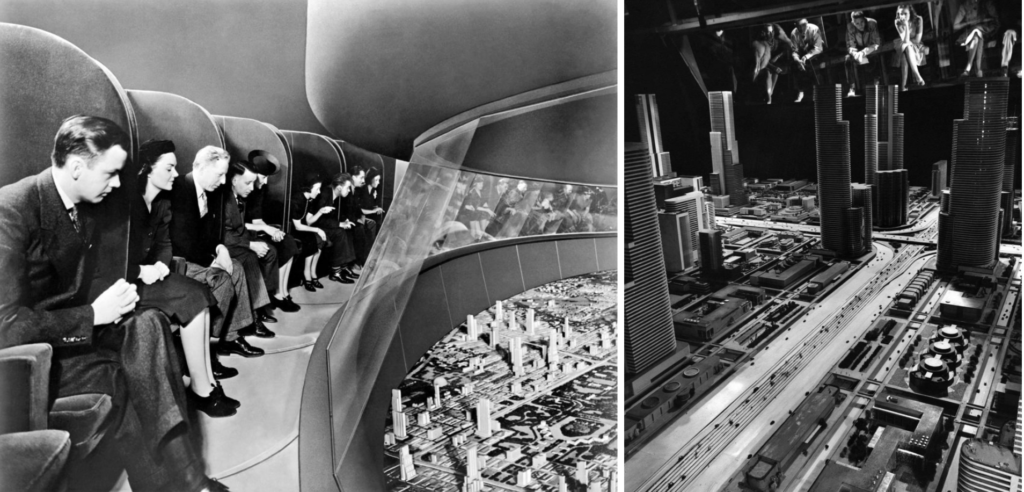
    The idea of a self-driving vehicle is very old. A magic flying carpet appears in The Book of the Thousand Nights and One Night and is attributed to the court of King Solomon. Leonardo da Vinci left a sketch of a clockwork cart that would go through a preprogrammed route. And so on, and so forth: I will refer to an excellent article by Marc Weber and steal only two photographs from there. Back in 1939, General Motors had a huge pavillion at the New York World’s Fair; in an aptly named Futurama ride (did Matt Groening take inspiration from General Motors?), they showed their vision of the cities of the future. These cities included smart roads that would inform smart vehicles, and they would drive autonomously with no supervision from humans. Here is how General Motors envisaged the future back in 1939:

    The reality still has not quite caught up with this vision, and the path to self-driving vehicles has been very slow. There were successful experiments with self-driving cars in the 1970s. in particular, in 1977 the Tsukuba Mechanical Engineering Laboratory in Japan developed a computer that would automatically steer a car based on visually distinguishable markers that city streets would have to be fitted with.

    In the 1980s, a project funded by DARPA produced a car that could actually travel along real roads using computer vision. This was the famous ALV (Autonomous Land Vehicle) project, and its vision system was able to locate roads in the images from cameras, solve the inverse geometry problem and send the three-dimensional road centerpoints to the navigation system. Here is how it worked:

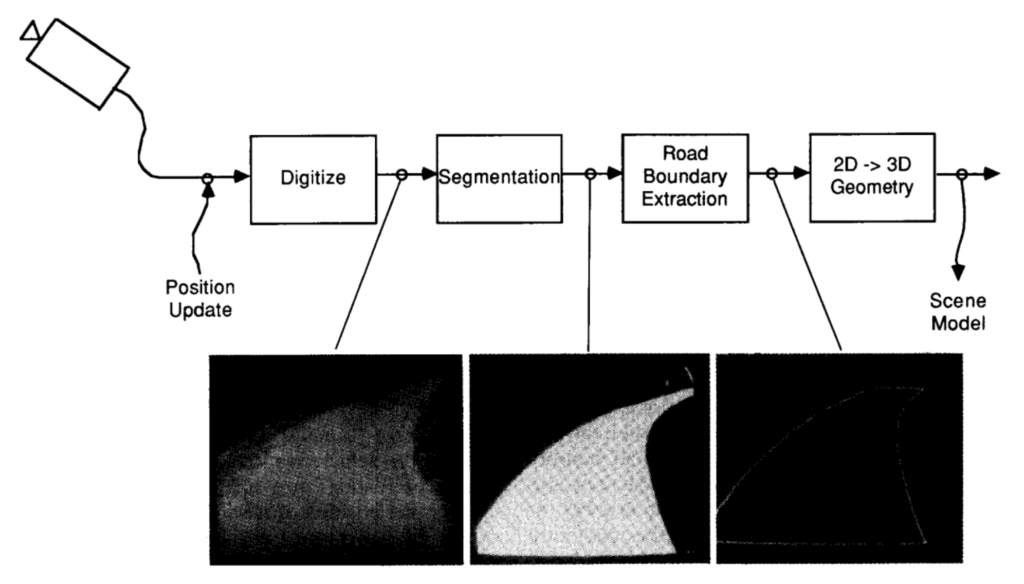
    The vision system, called VITS (for Vision Task Sequencer) and summarized in a paper by Turk et al. (the figures above and below are taken from there), did not use machine learning in the current meaning of the word. Similar to other computer vision systems of those days, as we discussed in the previous post, it relied on specially developed segmentation, road boundary extraction, and inverse geometry algorithms. The pipeline looked like this:

    How well did it all work? The paper reports that the ALV “could travel a distance of 4.2 km at speeds up to 10 km/h, handle variations in road surface, and navigate a sharp, almost hairpin, curve”. Then obstacle avoidance was added to the navigation system, and Alvin (that was the nickname of the actual self-driving car produced by the ALV project) could steer clear of the obstacles on a road and speed up to 20 km/h on a clear road. Pretty impressive for the 1980s, but, of course, the real problems (such as passengers jumping in front of self-driving cars) did not even begin to be considered.

    Putting the NN in ALVINN: a self-driving neural network in 1989

    Alvin did not learn, did not need any data, and therefore no synthetic data. Why are we talking about these early days of self-driving at all?

    Because this “no learning” stance changed very soon. In 1989, Dean A. Pomerleau published a paper on NIPS (this was the 2nd NIPS, a very different kind of conference than what it has blossomed into now) called ALVINN: An Autonomous Land Vehicle In a Neural Network. This was, as far as I know, one of the first attempts to produce computer vision systems for self-driving cars based on machine learning. And it had neural networks, too!

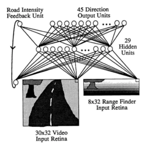
    The basic architecture of ALVINN was as follows:

    This means that the neural network had two kinds of input: 30 × 32 videos supplemented with 8 × 32 range finder data. The neural architecture was a classic two-layer feedforward network: input pixels go through a hidden layer and then on to the output units that try to tell what is the curvature of the turn ahead, so that the vehicle could stay on the road. There is also a special road intensity feedback unit that simply tells whether the road was lighter or darker than the background on the previous input image.

    The next step was to train ALVINN. To train, the network needed a training set. Here is what Dean Pomerleau has to say about the training data collection:

    Training on actual road images is logistically difficult, because in order to develop a general representation, the network must be presented with a large number of training exemplars depicting roads under a wide variety of conditions. Collection of such a data set would be difficult, and changes in parameters such as camera orientation would require collecting an entirely new set of road images…

    This is exactly the kind of problems with labeling and dataset representativeness that we discussed for modern machine learning, only Pomerleau is talking about these problems in 1989, in the context of 30 × 32 pixel videos! And what is his solution? Let’s read on:

    …To avoid these difficulties we have developed a simulated road generator which creates road images to be used as training exemplars for the network.

    Bingo! As soon as researchers needed to solve a real-world computer vision problem with a neural network, synthetic data appeared. This was one of the earliest examples of automatically generated synthetic datasets used to train an actual computer vision system.

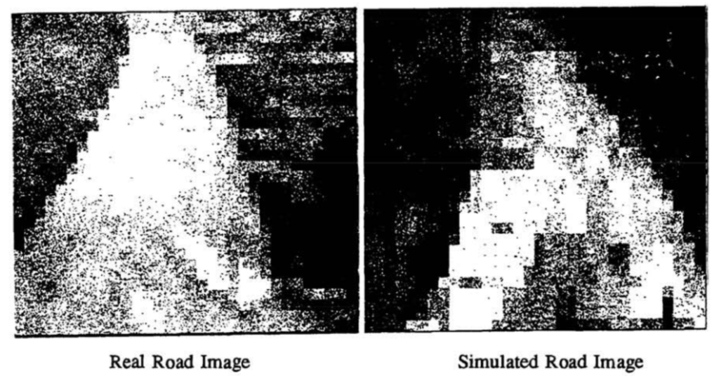
    Actually, low resolution of the sensors in those days made it easier to use synthetic data. Here are two images used by ALVINN, a real one on the left and a simulated one on the right:

    It doesn’t take much to achieve photorealism when the camera works like this, right?

    The results were positive. On synthetic test sets, ALVINN could correctly (within two units) predict turn curvature approximately 90% of the time, on par with the best handcrafted algorithms of the time. In real world testing, ALVINN could drive a car along a 400 meter path at a speed of half a meter per second. Interestingly, the limiting factor here was the speed of processing for the computer systems. Pomerleau reports that ALV’s handcrafted algorithms could achieve a speed of 1 meter per second, but only on a much faster Warp computer, while ALVINN was working on the on-board Sun computer, and he expects “dramatic speedups” after switching to Warp.

    I have to quote from Pomerleau’s conclusions again here — apologies for so many quotes, but this work really shines as a very early snapshot of everything that is so cool about synthetic data:

    Once a realistic artificial road generator was developed, back-propagation produced in half an hour a relatively successful road following system. It took many months of algorithm development and parameter tuning by the vision and autonomous navigation groups at CMU to reach a similar level of performance using traditional image processing and pattern recognition techniques.

    Pomerleau says this more as a praise for machine learning over handcrafted algorithm development, and that conclusion is correct as well. But it would take much more than half an hour if Pomerleau’s group had to label every single image from a real camera by hand. And of course, to train for different driving conditions they would need to collect a whole new dataset in the field, with a real car, rather than just tweak the parameters of the synthetic data generator. This quote is as much evidence for the advantages of synthetic data as for machine learning in general.

    What about now?

    But what if all this was this just a blip in the history of self-driving car development? Is synthetic data still used for this purpose?

    Of course, and much more intensely than in the 1980s. We will return to this in much more detail in this blog later; for now, let me just note that apart from training computer vision models for autonomous vehicles, synthetic data can also provide interactive simulated environments, where a driving agent can be trained by reinforcement learning (remember one of our previous posts), fine-tuning computer vision models and training the agent itself together, in an end-to-end fashion.

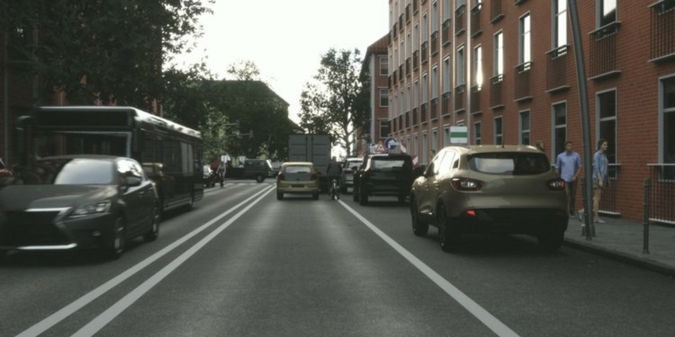
    The datasets themselves have also traveled a long way since the 30 × 32 videos of ALVINN. Again, we will return to this later in much more detail, for now I will just give you a taste. Here is a sample image from Synscapes, a recently published dataset with an emphasis on photorealism:

    I don’t think I would be of much use as a discriminator for images like this. The domain transfer problem, alas, still remains relevant… but that’s a topic for another day.

    Conclusion

    In this post, I have concentrated on a single specific application of synthetic data in computer vision: training self-driving cars. This was indeed one of the first fields where holistic approaches to training computer vision models from data proved their advantages over handcrafted algorithms. And as we have seen today, synthetic data was instrumental in this development and still remains crucial for autonomous vehicle models up to this day. Next time, we will move on to other robots.

    Sergey Nikolenko
    Head of AI, Synthesis AI
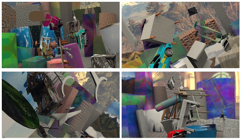
  • Synthetic Data: The Early Days, Part I

    Synthetic Data: The Early Days, Part I

    Previously on this blog, we have discussed the data problem: why machine learning may be hitting a wall, how one-shot and zero-shot learning can help, how come reinforcement learning does not need data at all, and how unlabeled datasets can inform even supervised learning tasks. Today, we begin discussing our main topic: synthetic data. Let us start from the very beginning: how synthetic data was done in the early days of computer vision…

    A brief intro to synthetic data

    Let me begin by reminding the general pipeline of most machine learning model development processes:

    Synthetic data is an important approach to solving the data problem by either producing artificial data from scratch or using advanced data manipulation techniques to produce novel and diverse training examples. The synthetic data approach is most easily exemplified by standard computer vision problems, and we will do so in this post too, but it is also relevant in other domains.

    In basic computer vision problems, synthetic data is most important to save on the labeling phase. For example, if you are solving the segmentation problem it is extremely hard to produce correct segmentation masks by hand. Here are some examples from the Microsoft COCO (Common Objects in Context) dataset:

    You can see that the manually produced segmentation masks are rather rough, and it is very expensive to make them much better if you need a large-scale dataset as a result.

    But suppose that all these scenes were actually 3D models, rendered in virtual environments with a 3D graphics engine. In that case, we wouldn’t have to painstakingly label every object with a bounding box or, even worse, a full silhouette: every pixel would be accounted for by the renderer and we would have all the labeling for free! What’s more, the renderer would provide useful labeling which is impossible for humans and which requires expensive hardware to get in reality, such as, e.g., depth maps (distance to camera) or surface normals. Here is a sample from the ProcSy dataset for autonomous driving:

    We will speak a lot more about synthetic data in this blog, but for now let us get on to the main topic: how synthetic data started its journey and what its early days looked like.

    The first steps: line drawings as synthetic data

    Computer vision started as a very ambitious endeavour. The famous “Summer Vision Project” by Seymour Papert was intended for summer interns and asked to construct a segmentation system, in 1966:

    Back in the 1960s and 1970s, usable segmentation on real photos was very hard to achieve. As a result, people turned to… synthetic data! I am not kidding, synthetic images in the form of artificial drawings are all over early computer vision.

    Consider, for example, the line labeling problem: given a picture with clearly depicted lines, mark which of the lines represent concave edges and which are convex. Here is a sample picture with this kind of labeling for two embedded parallelepipeds, taken from the classic paper by David Huffman, Impossible Objects as Nonsense Sentences:

    Figure (a) on the left shows a fully labeled “X-ray” image, and figure (b) shows only the visible part, but still fully labeled. And here is an illustration of a similar but different kind of labeling, this time from another classic paper by Max Clowes, On Seeing Things:

    Here Clowes distinguishes different types of corners based on how many edges form them and what kind of edges (concave or convex) they are. So basically it’s the same problem: find out the shape of a polyhedron defined as a collection of edges projected on a plane, i.e., shown as a line drawing.

    Both Huffman and Clowes work (as far as I understand, independently) towards the goal of developing algorithms for this problem. They address it primarily as a topological problem, use the language of graph theory and develop conditions under which a 2D picture can correspond to a feasible 3D scene. They are both fascinated with impossible objects, 2D drawings that look realistic and satisfy a lot of reasonable necessary conditions for realistic scenes but at the same time still cannot be truly realized in 3D space. Think of M.C. Escher’s drawings (on the left, a fragment from “Ascending and descending”) or the famous Penrose triangle (on the right):

    And here are two of the more complex polyhedral shapes, the one on the left taken from Huffman and on the right, from Clowes. They are both impossible but it’s not so easy to spot it by examining local properties of their graphs of lines:

    But what kind of examples did Huffman and Clowes use for their test sets? Well, naturally, it proved to be way too hard for the computer vision of the 1960s to extract coherent line patterns like these from real photographs. Therefore, this entire field was talking about artificially produced line drawings, one of the first and simplest examples of synthetic data in computer vision.

    Synthetic data for a quantitative comparison

    In the early days of computer vision, many problems were tackled not by machine learning but by direct attempts to develop algorithms for specific tasks. Let us take as the running example the problem of measuring optical flow. This is one of the basic low-level computer vision problems: estimate the distribution of apparent velocities of movement along the image. Optical flow can help find moving objects on the image or estimate (and probably subtract) the movement of the camera itself, but its most common use is for stereo matching: by computing optical flow between images taken at the same time from two cameras, you can match the picture in stereo and then do depth estimation and a lot of scene understanding. In essence, optical flow is a field of vectors that estimate the movement of every pixel between a pair of images. Here is an example (taken from here):

    The example above was produced by the classical Lucas-Kanade flow estimation algorithm. Typical for early computer vision, this is just an algorithm, there are no parameters to be learned from data and no training set. In their 1981 paper, Lucas and Kanade do not provide any quantitative estimates for how well their algorithm works, they just give several examples based on a single real world stereo pair. Here it is, by the way:

    And this is entirely typical: all early works on optical flow estimation develop and present new algorithms but do not provide any means for a principled comparison beyond testing them on several real examples.

    When enough algorithms had been accumulated, however, the need for an honest and representative comparison became really pressing. For an example of such a comparison, we jump forward to 1994, to the paper by Barron et al. called Performance of Optical Flow Techniques. They present a taxonomy and survey of optical flow estimation algorithms, including a wide variety of differential (such as Lucas-Kanade), region-based, and energy-based methods. But to get a fair experimental comparison, they needed a test set with known correct answers. And, of course, they turned to synthetic data for this. They concisely sum up the pluses and minuses of synthetic data that remain true up to this day:

    The main advantages of synthetic inputs are that the 2-D motion fields and scene properties can be controlled and tested in a methodical fashion. In particular, we have access to the true 2-D motion field and can therefore quantify performance. Conversely, it must be remembered that such inputs are usually clean signals (involving no occlusion, specularity, shadowing, transparency, etc.) and therefore this measure of performance should be taken as an optimistic bound on the expected errors with real image sequences.

    For the comparison, they used sinusoidal inputs and a moving dark square over a bright background:

    They also used synthetic camera motion: take a still real photograph and start cropping out a moving window over this image, and you get a camera moving perpendicular to its line of sight. And if you take a window and start expanding it, you get a camera moving outwards:

    These synthetic data generation techniques were really simple and may seem naive by now, but they did allow for a reasonable quantitative comparison: it turned out that even on such seemingly simple inputs the classical optical flow estimation algorithms gave very different answers, with widely varying accuracy.

    Conclusion

    Today, we saw two applications of synthetic data in early computer vision. First, simple line drawings suffice to present an interesting challenge for 3D scene understanding, even when interpreted as precise polyhedra. Second, while classical algorithms for low-level computer level problems almost never involved any learning of parameters, to make a fair comparison you need a test set with known correct answers, and this is exactly where machine learning can step up. But stay tuned, that’s not all, folks! See you next time!

    Sergey Nikolenko
    Head of AI, Synthesis AI
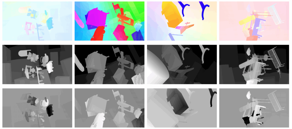
  • The Data Problem IV: Can Unlabeled Data Help?

    The Data Problem IV: Can Unlabeled Data Help?

    In the first three posts of this series, we have seen several ways to overcome the data problem in machine learning: first we posed the problem, then discussed one-shot and zero shot learning, and in the third post presented the reinforcement learning way of using no data at all. In this final installment, we discuss the third direction that modern machine learning takes to help with the lack of labeled data: how can we use unlabeled data to help inform machine learning models?

    Source: https://www.kickstarter.com/projects/1323560215/unlabeled-the-blind-beer-tasting-game/posts/2076400

    Why Can Unlabeled Data Be Useful?

    For many problems, obtaining labeled data is expensive but unlabeled data, especially data that is not directly related to the problem, is plentiful. Consider the computer vision problems we talked about above: it’s very expensive to get a large dataset of labeled images of faces, but it’s much less expensive to get a large dataset of unlabeled such images, and it’s almost trivial to just get a lot of images with and without faces.

    But can they help? Basic intuition tells that it may not be easy but should be possible. After all, we humans learn from all sorts of random images and get an intuition about the world around us that generalizes exceedingly well. Armed with this intuition, we can do one-shot and zero-shot learning with no problem. And the images were never actually labeled, our learning can hardly be called supervised.

    In machine learning, the intuition is similar. Suppose you want to teach a model to tell cats and dogs apart on one-megapixel photos. Mathematically speaking, each photo is a vector of about 3 million real values (RGB values for every pixel; they are in fact discretized but we will forgo this part), and our problem is to construct a decision surface in the space R3,000,000 (sounds formidable, right?). Obviously, random points in this space will look like white noise on the image; “real photos”, i.e., photos that we can recognize as something from the world around us, form a very low-dimensional, at least compared to 3 million, manifold in this space (I am using the word “manifold” informally, but it probably really is an open subset: if you take a realistic photo and change one pixel or change every pixel by a very small value, the photo will remain realistic). Something like the picture we already saw in the first installment of this series:

    Source: https://nlp.stanford.edu/~socherr/SocherGanjooManningNg_NIPS2013.pdf

    It is now not surprising that the main problem a machine learning model faces in real life computer vision is not to separate cats from dogs given a good parametrization of this extremely complicated manifold but to learn the parametrization (i.e., parameter structure) itself. And to learn this manifold, unlabeled data is just as useful as labeled data: we are trying to understand what the world looks like in general before we label and separate individual objects.

    Although it’s still a far cry from human abilities (see this recent treatise by Francois Chollet for a realistic breakdown of where we stand in terms of general AI), there are several approaches being developed in machine learning to make use of all this extra unlabeled data lying around. Let us consider some of them.

    Weakly Supervised Training: Trading Labels for Computation

    The first way is to use unlabeled data to produce new labeled data. The idea is similar to the EM algorithm: let’s assign labels to images where we don’t have them with imperfect models trained on what labeled data we have. Although we won’t be as sure that the labels are correct, they will still help, and we will revisit and correct them on later iterations. In a recent paper (Xie et al., 2019), researchers from Google Brain and Carnegie Mellon University applied the following algorithm:

    • start from a “teacher” model trained as usual, on a (smaller) labeled dataset;
    • use the “teacher” model on the (larger) unlabeled dataset, producing pseudolabels;
    • train a “student” model on the resulting large labeled dataset;
    • use the student model as a teacher for the next iteration, rinse and repeat.

    While this is a rather standard approach, used many times before in semi-supervised learning, by smartly adding noise to the student model Xie et al. managed to improve state of the art results on ImageNet, the most standard and beaten-down large-scale image classification dataset.

    For this, however, they needed a separate dataset with 300 million unlabeled images and a lot of computational power (3.5 days on a 2048-core Google TPU, on the same scale as needed to train AlphaZero to beat everybody in Go and chess; last time we discussed how these experiments have been estimated to cost about $35 million to replicate).

    Cut-and-Paste Models for Unsupervised Segmentation

    Another interesting example of replacing labeled data with (lots of) unlabeled comes from a very standard computer vision problem: segmentation. It is indeed very hard to produce labeled data for training segmentation models (we discussed this in the first post of the series)… but do we have to? If we go back to segmentation models from classical computer vision, they don’t require any labeled data: they cluster pixels according to their features (color and perhaps features of neighboring pixels) or run an algorithm to cut the graph of pixels into segments with minimal possible cost. Modern deep learning models work much better, of course, but it looks like recent advances make it possible to train deep learning models to do segmentation without labeled data as well.

    Approaches such as W-Net (Xia, Kulis, 2017) use unsupervised autoencoder-style training to extract features from pixels and then segment them with a classical algorithm. Approaches such as invariant information clustering (Ji et al., 2019) develop image clustering approaches and then apply them to each pixel in a convolution-based way, thus transforming image clustering into segmentation.

    One of the most intriguing lines of work that results in unsupervised clustering uses GANs for image manipulation. The “cut-and-paste” approach (Remez et al., 2018) works in an adversarial way:

    • one network, the mask generator, constructs a segmentation mask from the features of pixels in a detected object;
    • then the object is cut out according to this mask and transferred to a different, object-free location on the image;
    • another network, the discriminator, now has to distinguish whether an image patch has been produced by this cut-and-paste pipeline or is just a patch of a real image.

    The idea is that good segmentation masks will make for realistic pasted images, and in order to convince the discriminator the mask generator will have to learn to produce high-quality segmentation masks. Here is an illustration:

    A bad mask (a) produces a very unconvincing resulting image (b), while a good segmentation mask (c) makes for a pasted image (d) which is much harder to distinguish from a real image (e).

    The same effect appeared in a paper where I participated recently. The SEIGAN (Segment-Enhance-Inpaint GAN) model (Ostyakov et al., 2019) has been designed for compositional image generation, learning to transfer objects from one image to another in a convincing way. Similar to the cut-and-paste approach above, as a side effect of the SEIGAN model we obtained high-quality unsupervised segmentation! I won’t go into details, but here is an illustration of the SEIGAN pipeline:

    In this pipeline, segmentation is needed to cut out the object that we’d like to transfer. The network never receives any correct segmentation masks for training. It learns in a GAN-based way, by training to fool discriminators that try to tell images with transferred objects apart from real images (I simplify a bit, actually there are plenty of loss functions in SEIGAN in addition to the adversarial loss, but still no supervision), so segmentation comes for free, as a “natural” way to cut out objects. Perhaps that’s not unlike how we learned to do segmentation when we were infants.

    Semi-supervised teacher-student training and unsupervised segmentation via cut-and-paste are just two directions out of many that are currently being developed. In these works, researchers are exploring various ways to trade the need for labeled datasets for extra unlabeled data, extra unrelated data, or extra computation, all of which is becoming more and more readily available. I am sure we will hear much more about “unsupervised X” in the future, where X might take the most unexpected values.

    Conclusion

    It is time to sum up the series. Faced with the lack of labeled data in many applications, machine learning researchers have been looking for ways to solve problems without sufficiently large labeled datasets available. We have discussed three basic ideas that have already blossomed into full-scale research directions:

    • one-shot and zero-shot learning that allow models to quickly extend themselves to new classes with very little new labeled data;
    • reinforcement learning that often needs no data at all beyond an environment that constitutes the “rules of the game”;
    • weakly supervised learning that informs supervised models with large amounts of unlabeled data.

    As you might have guessed from the name of the company, Synthesis AI presents a different way to tackle the data problem: synthetic data. In this approach, models are trained on automatically generated data, where labels usually come for free after a one-time upfront investment of labor into creating the synthetic simulation. We specialize in creating synthetic environments and objects, producing synthetic labeled datasets for various problems, and solving the domain transfer and domain adaptation problems, where models trained on synthetic data need to be transferred to operate on real photos.

    Next time, we will speak more about synthetic data in modern machine learning. Stay tuned!

    Sergey Nikolenko
    Head of AI, Synthesis AI

  • The Data Problem III: Machine Learning Without Data

    The Data Problem III: Machine Learning Without Data

    Today, we continue our series on the data problem in machine learning. In the first post, we realized that we are already pushing the boundaries of possible labeled datasets. In the second post, we discussed one way to avoid huge labeling costs: using one-shot and zero-shot learning. Now we are in for a quick overview of the kind of machine learning that might go without data at all: reinforcement learning.

    Reinforcement Learning: Beating the Pros With No Data

    Interestingly, some kinds of machine learning do not require any external data at all, let alone labeled data. Usually the idea is that they are able to generate data for themselves.

    The main field where this becomes possible is reinforcement learning (RL), where an agent learns to perform well in an interactive environment. An agent can perform actions and receive rewards for these actions from the environment. Usually, modern RL architectures consist of the feature extraction part that processes environment states into features and an RL agent that transforms features into actions and converts rewards from the environment into weight updates. Here is a flowchart from a recent survey of deep RL for video games (Shao et al., 2019):

    In the space of a short blog post it is, of course, impossible to do justice to a wide and interesting field such as reinforcement learning. So before we proceed to the main point of this post, let me only mention that for a long time, RL had been a very unusual field of machine learning in that the best introductory book in RL had been written twenty years ago. It was the famous book by Richard S. Sutton and Andrew G. Barto, Reinforcement Learning: An Introduction, first published in 1998. Naturally, it could not contain anything about the recent deep learning revolution that has transformed RL as well. Fortunately, very recently Sutton and Barto have published the second edition of their book. It’s still as well-written and accessible to beginners but now it contains the modern ideas as well; what’s more, it is available for free.

    The poster child of modern data-free approaches to RL is AlphaZero by DeepMind (Silver et al., 2018). Their original breakthrough was AlphaGo (Silver et al., 2016), a model that beat Lee Sedol, one of the top human Go players. Long after DeepBlue beat Kasparov in chess, professional-level Go was remaining out of reach for computer programs, and AlphaGo’s success was unexpected even in 2016.

    The match between Lee Sedol and AlphaGo became one of the most publicized events in AI and was widely considered as the “Sputnik moment” for Asia in AI, the moment when China, Japan, and Korea realized that deep learning is to be taken seriously. Lee Sedol (on the left below) could win one of the games, so although at the moment he was discouraged by losing to AlphaGo, I decided to illustrate this with what I believe to be the last serious game of Go won by humans against top computer players. When Ke Jie (on the right below), then #1 in the world Go rankings, played against an updated AlphaGo model two years later, he admitted that he did not stand a chance at any point:
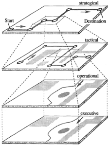
    But AlphaGo utilized a lot of labeled data: it had a pretraining step that used a large database of professional games. AlphaZero takes its name from the fact that it needs zero training data: it begins by knowing only the rules of the game and achieves top results through self-play, actually with a very simple loss function combined with tree search. AlphaZero beat AlphaGo (and its later version, AlphaGo Zero) in Go and one of the top chess engines, Stockfish, in chess.

    The latest result by the DeepMind RL team, MuZero (Schrittweiser et al., 2019), is even more impressive. MuZero represents model-based RL, that is, it builds a model of the environment as it goes and does not know the rules of the game beforehand but has to learn them from scratch; e.g., in chess it cannot make illegal moves as actions but can consider them in tree search and has to learn that they are illegal by itself. With this additional complication, MuZero was able to achieve AlphaZero’s skill in chess and shogi and even outperform it in Go. Most importantly, the same model could also be applied to, e.g., computer games in Atari environments (a standard benchmark in reinforcement learning).

    So what’s the catch? One problem is that not every problem can be formulated in terms of RL with no data required. You can learn to play games, i.e., self-contained finite structures where all rules are known in advance. But how do we learn, say, autonomous driving or walking, with a much wider variety of possible situations and individual components of these situations? One possible solution is to use synthetic virtual environments; let us proceed to a very interesting example of reinforcement learning for robotics.

    Solving the Rubik’s Cube: The Story of Dactyl

    One of the main fields of application for reinforcement learning is robotics: a field where machine learning models need to learn to perform in a real physical environment. From autonomous cars to industrial robotic arms, these environments are united by two properties.

    • It is impossible to collect a labeled dataset for the robot: we can tell whether it has succeeded in solving the task (this will be the reward), but we do not have a dataset of which “muscles” to “flex” in order to successfully play ping-pong or fly a drone. This is the main reason why RL is so important for robotics. Before RL, robots were programmed by hand by solving optimal control problems, but solutions based on reinforcement learning prove to be much better and more robust.
    • At the same time, using reinforcement learning directly, like AlphaZero does, is impossible because the robot does not have the luxury of spending thousands of real years training. This reason leads to using synthetic virtual environments for robotics, where it is actually possible to have millions of training runs.

    Again, in this blog post we cannot hope to cover everything related to virtual environments for robotics; for a more detailed exposition see my recent survey (Nikolenko, 2019). I will only tell one story: the story of how a dexterous manipulation robot has learned to solve the Rubik’s cube.

    The robot is a product of OpenAI, a famous company that drives research in many areas of machine learning, RL being a primary goal. In 2019, OpenAI has also produced OpenAI Five, a model that beat professionals in DotA 2, and earlier they had released OpenAI Gym, the main testing environment for reinforcement learning models.
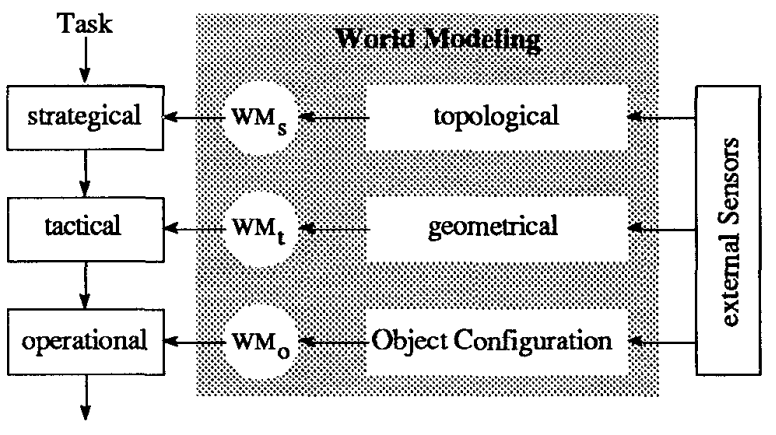
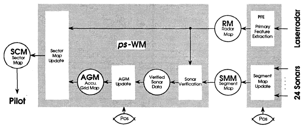
    Dactyl, the robot that we are talking about, is a longstanding project in OpenAI, initiated in 2016. The first big result came in 2018, when their robotic hand learned the basics of dexterous manipulation (OpenAI et al, 2018). In particular, they learned to take a block with letters and rotate it so that the target letter faces camera:

    This was already a marvelous achievement. I will not go into the details of the robotic environment, the hand itself, or reinforcement learning algorithms that learned to do this. The main point for us is that they did not use any kind of domain adaptation techniques: they trained the robot entirely in a virtual environment and it worked almost seamlessly in real life.

    To make it work, one has to apply domain randomization. The idea is to make synthetic data so varied that in order to succeed the model will have to be very robust. So robust that the distribution of environments where it works well will also cover the real world. The OpenAI team varied many parameters of the environment, including visual parameters such as and physical parameters such as size and weight of the cube, friction coefficients on the surfaces and in the robot’s joints, and so on. Here is a sample of their different visualizations:

    With this kind of domain randomization, they were able to learn to rotate blocks. But they wanted to solve Rubik’s cube! The previous synthetic environment somehow did not lead to success on this task. There is a tradeoff in the use of synthetic data here: if the variance in environmental parameters is too big, so the environment is too different every time, it will be much harder for the algorithm to make any progress at all.

    Therefore, in their next paper (Akkaya et al., 2019) the authors modified the synthetic environment and made it grow in complexity with time. That is, the parameters of synthetic data generation (size of the cube, friction forces and so on) are at first randomized within small ranges, and these ranges grow as training progresses:

    This idea, which the OpenAI team called automatic domain randomization (ADR), is an example of the “closing the feedback loop” idea that we are pursuing here at Synthesis AI: make the results of the model trained on synthetic data drive the generation of new synthetic data. Note how even a small step in this direction—the feedback here is limited to overcoming a given threshold that triggers the next step in the curriculum of changing synthetic data parameters—significantly improves the results of the model. The resulting robotic hand is stable even to perturbations that had never been part of the synthetic environment; it is unfazed even by the notorious plush giraffe:

    Leaving Moore’s Law in the Dust

    So are we done with datasets in machine learning, then? Reinforcement learning seems to achieve excellent results and keeps beating state of the art with no labeled data at all or at the one-time expense of setting up the synthetic environment. Unfortunately, there is yet another catch here.

    The problem, probably just as serious as the lack of labeled data, is the ever-growing amount of computation needed for further advances in reinforcement learning. To learn to play chess and Go, MuZero used 1000 third generation Google TPUs to simulate self-play games. This doesn’t tell us much by itself, but here is an interesting observation made by OpenAI (OpenAI blog, 2018; see also an addendum from November 2019). They noticed that before 2012, computational resources needed to train state of the art AI models grew basically according to Moore’s Law, doubling the computational requirements every two years. But with the advent of deep learning, in 2012-2019 computational resources for top AI training doubled on average every 3.4 months!

    This is a huge rate of increase, and, obviously, it cannot continue forever, as the actual hardware computational power growth is only slowing down compared to Moore’s Law. The AlphaZero paper contains two experiments; the smaller one has been estimated to cost about $3 million to replicate on Google Cloud at 2019 prices, and the large experiment costs upwards of $30 million (Huang, 2019). While the cost of computation is dropping, it does so at a much slower rate than the increase of computation needed for AI.

    Thus, one possible scenario for further AI development is that yes, indeed, this “brute force” approach might theoretically take us very far, maybe even to general artificial intelligence, but it would require more computational power than we actually have in our puny Solar System. Note that a similar thing, albeit on a smaller scale, happened with the second wave of hype for artificial neural networks: researchers in the late 1980s had a lot of great ideas about neural architectures (we had CNNs, RNNs, RL and much more), but neither the data nor the computational power was sufficient to make a breakthrough, and neural networks were relegated to “the second best way to do almost anything”.

    Still, at present reinforcement learning represents another feasible way to trade labeled data for computation, as the example of AlphaGo blossoming into AlphaZero and MuZero clearly shows.

    Conclusion

    In this post, we have discussed a way to overcome the need for ever-increasing labeled datasets. In problems that can be solved by reinforcement learning, it often happens that the model either does not need labeled data at all or needs a one-time investment in a synthetic virtual environment. However, it turns out that successes in reinforcement learning come at a steep computational cost, perhaps too steep to continue even in the nearest future.

    Next time, we will discuss another way to attack the data problem: using unlabeled datasets to inform machine learning models and help reduce the requirements for labeling. This will be the last preliminary post before we dive into the main topic of this blog and our company: synthetic data.

    Sergey Nikolenko
    Head of AI, Synthesis AI