In this (very) long post, we present an entire whitepaper on synthetic data, proving that synthetic data works even without complicated domain adaptation techniques in a wide variety of practical applications. We consider three specific problems, all related to human faces, show that synthetic data works for all three, and draw some other interesting and important conclusions.
Introduction
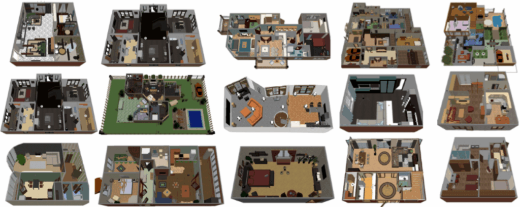
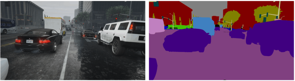
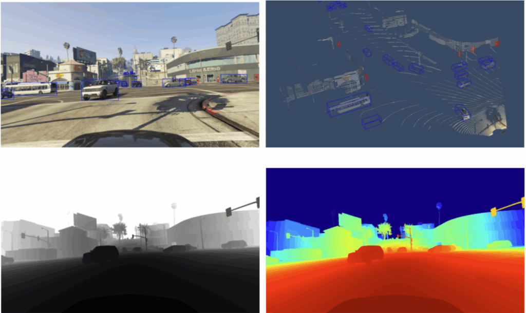
Synthetic data is an invaluable tool for many machine learning problems, especially in computer vision, which we will concentrate on below. In particular, many important computer vision problems, including segmentation, depth estimation, optical flow estimation, facial landmark detection, background matting, and many more, are prohibitively expensive to label manually.
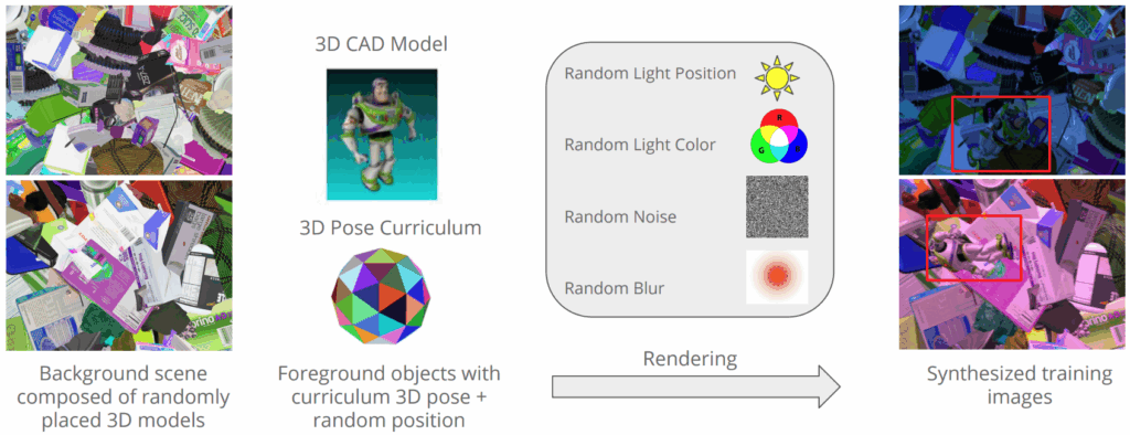
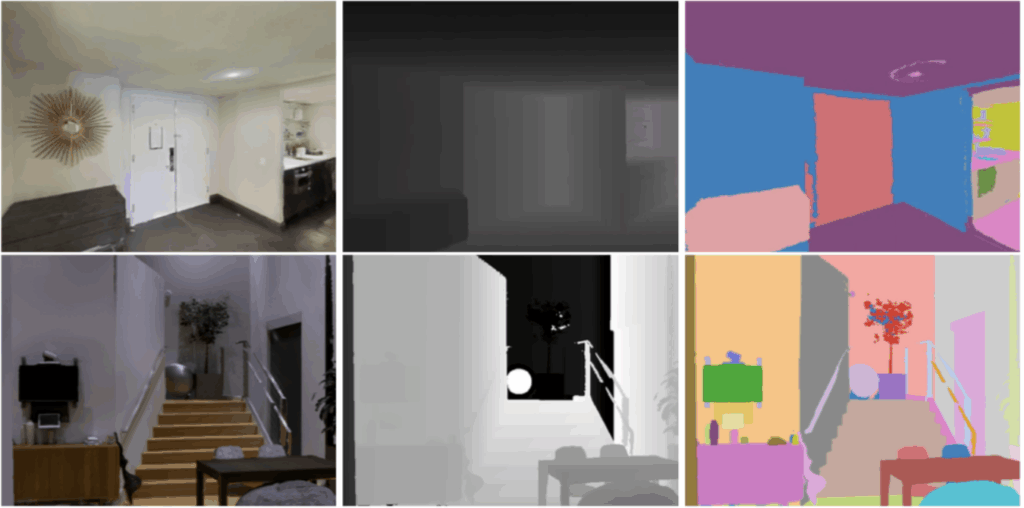
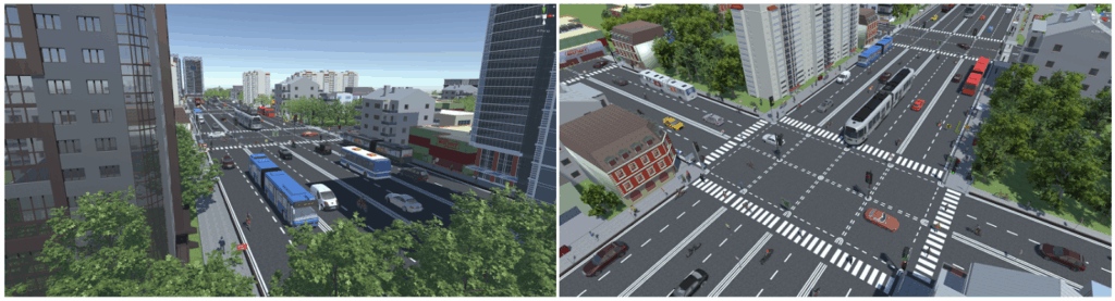
Synthetic data provides a way to have unlimited perfectly labeled data at a fraction of the cost of manually labeled data. With the 3D models of objects and environments in question, you can create an endless stream of data with any kind of labeling under different (randomized) conditions such as composition and placement of objects, background, lighting, camera placement and parameters, and so on. For a more detailed overview of synthetic data, see (Nikolenko, 2019).
Naturally, artificially produced synthetic data cannot be perfectly photorealistic. There always exists a domain gap between real and synthetic datasets, stemming both from this lack of photorealism and also in part from different approaches to labeling: for example, manually produced segmentation masks are generally correct but usually rough and far from pixel-perfect.
Therefore, most works on synthetic data center around the problem of domain adaptation: how can we close this gap? There exist approaches that improve the realism, called synthetic-to-real refinement, and approaches that impose constraints on the models—their feature space, training process, or both—in order to make them operate similarly on both real and synthetic data. This is the main direction of research in synthetic data right now, and much of recent research is devoted to suggesting new approaches to domain adaptation.
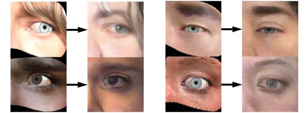
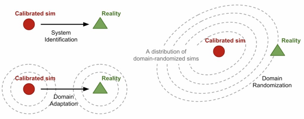
However, CGI-based synthetic data becomes better and better with time, and some works also suggest that domain randomization, i.e., simply making the synthetic data distribution sufficiently varied to ensure model robustness, may work out of the box. On the other hand, recent advances in related problems such as style transfer (synthetic-to-real refinement is basically style transfer between the domains of synthetic and real images) suggest that refinement-style domain adaptation may be done with very simple techniques; it might happen that while these techniques are insufficient for photorealistic style transfer for high-resolution photographs they are quite enough to make synthetic data useful for computer vision models.
Still, it turns out that synthetic data can provide significant improvements even without complicated domain adaptation approaches. In this whitepaper, we consider three specific use cases where we have found synthetic data to work well under either very simple or no domain adaptation at all. We are also actively pursuing research on domain adaptation, and ideas coming from modern style transfer approaches may prove to bring new interesting results here as well; but in this document, we concentrate on very straightforward applications of synthetic data and show that synthetic data can just work out of the box. In one of the case studies, we compare two main techniques to using synthetic data in this simple way—training on hybrid datasets and fine-tuning on real data after pretraining on synthetic—also with interesting results.
Here at Synthesis AI, we have developed the Face API for mass generation of high-quality synthetic 3D models of human heads, so all three cases have to do with human faces: face segmentation, background matting for human faces, and facial landmark detection. Note that all three use cases also feature some very complex labeling: while facial landmarks are merely very expensive to label by hand, manually labeled datasets for background matting are virtually impossible to obtain.
Before we proceed to the use cases, let us describe what they all have in common.
Data Generation and Domain Adaptation
In this section, we describe the data generation process and the synthetic-to-real domain adaptation approach that we used throughout all three use cases.
Face API by Synthesis AI
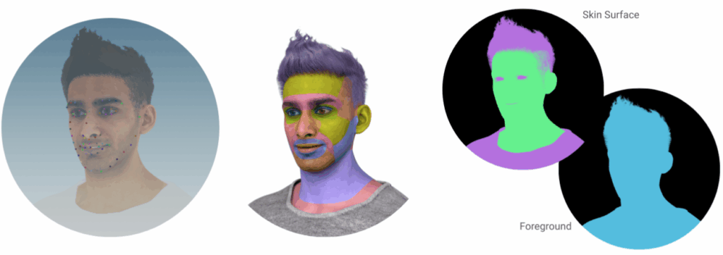
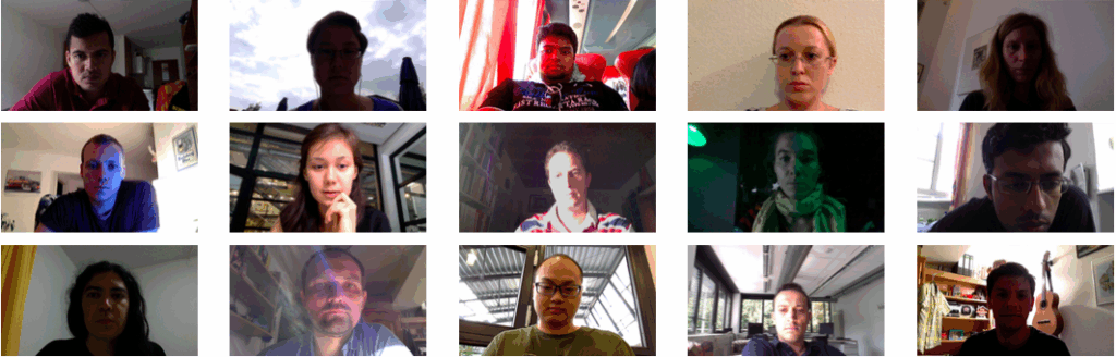
The Face API, developed by Synthesis AI, can generate millions of images comprising unique people, with expressions and accessories, in a wide array of environments, with unique camera settings. Below we show some representative examples of various Face API capabilities.
The Face API has tens of thousands of unique identities that span the genders, age groups, and ethnicity/skin tones, and new identities are added continuously. These
It also allows for modifications to the face, including expressions and emotions, eye gaze, head turn, head & facial hair, and more:
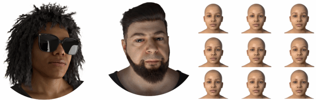
Furthermore, the Face API allows to adorn the subjects with accessories, including clear glasses, sunglasses, hats, other headwear, headphones, and face masks.

Finally, it allows for indoor & outdoor environments with accurate lighting, as well as additional directional/spot lighting to further vary the conditions and emulate reality.
The output includes:
- RGB Images
- Pupil Coordinates
- Facial Landmarks (iBug 68-like)
- Camera Settings
- Eye Gaze
- Segmentation Images & Values
- Depth from Camera
- Surface Normals
- Alpha / Transparency
Full documentation can be found at the Synthesis AI website. For the purposes of this whitepaper, let us just say that Face API is a more than sufficient source of synthetic human faces with any kind of labeling that a computer vision practitioner might desire.
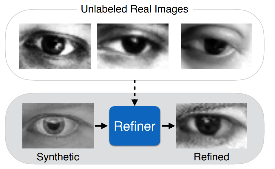
Synthetic-to-Real Refinement by Instance Normalization
Below, we consider three computer vision problems where we have experimented with using synthetic data to train more or less standard deep learning models. Although we could have applied complex domain adaptation techniques, we instead chose to use one simple idea inspired by style transfer models. Here we show some practical and less computationally intensive approaches that can work well too.
Most recent works on style transfer, including MUNIT (Huang et al., 2018), StyleGAN (Karras et al., 2018), StyleGAN2 (Karras et al., 2019), and others, make use of the idea of adaptive instance normalization (AdaIN) proposed by Huang and Belongie (2017).
The basic idea of AdaIN is to substitute the statistics of the style image in place of the batch normalization (BN) parameters for the corresponding BN layers during the processing of the content image:
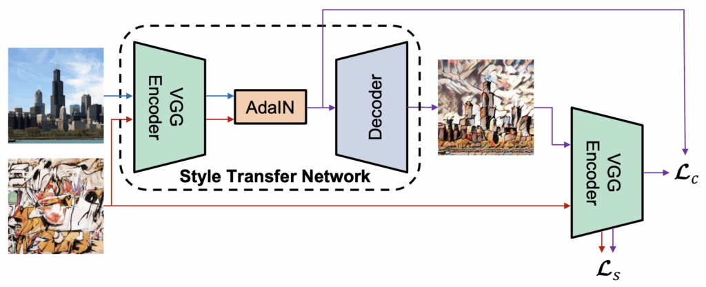
This is a natural extension of an earlier idea of conditional instance normalization (Dimoulin et al., 2016) where BN parameters were learned separately for each style. Both conditional and adaptive instance normalization can be useful for style transfer, but AdaIN is better suited for common style transfer tasks because it only needs a single style image to compute the statistics and does not require pretraining or, generally speaking, any information regarding future styles in advance.
In style transfer architectures such as MUNIT or StyleGAN, AdaIN layers are used as a key component for a complex involved architecture that usually also employs CycleGAN (Zhu et al., 2017) and/or ProGAN (Karras et al., 2017) ideas. As a result, these architectures are hard to train and, what is even more important, require a lot of computational resources to use. This makes state of the art style transfer architectures unsuitable for synthetic-to-real refinement since we need to apply them to every image in the training set.
However, style transfer results already in the original work on AdaIN (Huang and Belongie, 2017) already look quite good, and it is possible to use AdaIN in a much simpler architecture than state of the art style transfer. Therefore, in our experiments we use a similar approach for synthetic-to-real refinement, replacing BN statistics for synthetic images with statistics extracted from real images.
This approach has been shown to work several times in literature, in several variations (Li et al., 2016; Chang et al., 2019) We follow either Chang et al. (2019), which is a simpler and more direct version, or the approach introduced by Seo et al. (2020), called domain-specific optimized normalization (DSON), where for each domain we maintain batch normalization statistics and mixture weights learned on the corresponding domain:
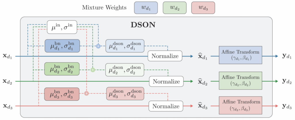
Thus, we have described our general approach to synthetic-to-real domain adaptation; we used it in some of our experiments but note that in many cases, we did not do any domain adaptation at all (these cases will be made clear below). With that, we are ready to proceed to specific computer problems.
Face Segmentation with Synthetic Data: Syn-to-Real Transfer As Good As Real-to-Real Transfer
Our first use case deals with the segmentation problem. Since we are talking about applications of our Face API, this will be the segmentation of human faces. What’s more, we do not simply cut out the mask of a human face from a photo but want to segment different parts of the face.
We have used two real datasets in this study:
- LaPa (Landmark guided face Parsing dataset), presented by Liu et al. (2020), contains more than 22,000 images, with variations in pose and facial expression and also with some occlusions among the images; it contains facial landmark labels (which we do not use) and faces segmented into 11 classes, as in the following example:
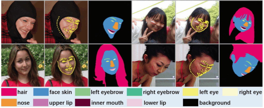
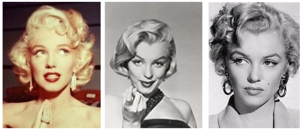
- CelebAMask-HQ, presented by Lee et al. (2019), contains 30,000 high-resolution celebrity face images with 19 segmentation classes, including various hairstyles and a number of accessories such as glasses or hats:


For the purposes of this study, we reduced both datasets to 9 classes (same as LaPa but without the eyebrows). As synthetic data, we used 200K diverse images produced by our Face API; no domain adaptation was applied in this case study (we have tried it and found no improvement or even some small deterioration in performance metrics).
As the basic segmentation model, we have chosen the DeepLabv3+ model (Chen et al., 2018) with the DRN-56 backbone, an encoder-decoder model with spatial pyramid pooling and atrous convolutions. DeepLabv3+ produces good results, often serves as a baseline in works on semantic segmentation, and, importantly, is relatively lightweight and easy to train. In particular, due to this choice all images were resized down to 256p.
The results, summarized in the table below, confirmed our initial hypothesis and even outperformed our expectations in some respects. The table shows the mIoU (mean intersection-over-union) scores on the CelebAMask-HQ and LaPa test sets for DeepLabv3+ trained on real data only from CelebAMask-HQ, mixed with synthetic data in various proportions.
In the table below, we show the results for different proportions of real data (CelebAMask-HQ) in the training set, tested on two different test sets.
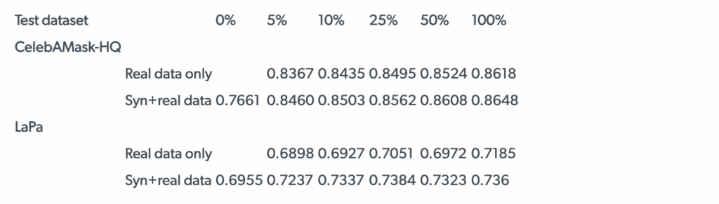
First of all, as expected, we found that training on a hybrid dataset with both real and synthetic data is undoubtedly beneficial. When both training and testing on CelebAMask-HQ (first two rows in the table), we obtain noticeable improvements across all proportions of real and synthetic data in the training set. The same holds for the two bottom rows in the table that show the results of DeepLabv3+ trained on CelebAMask-HQ and tested on LaPa.
But the most interesting and, in our opinion, important result is that in this context, domain transfer across two (quite similar) real datasets produces virtually the same results as domain transfer from synthetic to real data: results on LaPa with 100% only real data are almost identical to the results on LaPa with 0% real and only synthetic data. Let us look at the plots below and then discuss what conclusions we can draw:
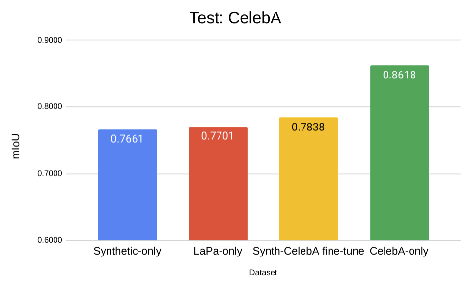
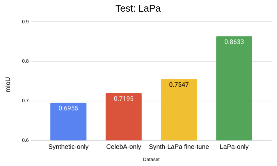
Most importantly, note that the domain gap on the CelebA test set amounts to a 9.6% performance drop for the Syn-to-CelebA domain shift and 9.2% for the LaPa-to-CelebA domain shift. This very small difference suggests that while domain shift is a problem, it is not a problem specifically for the synthetic domain, which performs basically the same as a different domain of real data. The results on the LaPa test set tell a similar story: 14.4% performance drop for CelebA-to-LaPa and 16.8% for Syn-to-LaPa.
Second, note the “fine-tune” bars that exhibit (quite significant) improvements over other models trained on a different domain. This is another effect we have noted in our experiments: it appears that fine-tuning on real data after pretraining on a synthetic dataset often works better than just training on a mixed hybrid syn-plus-real dataset.
Below, we show a more detailed look into where the errors are:
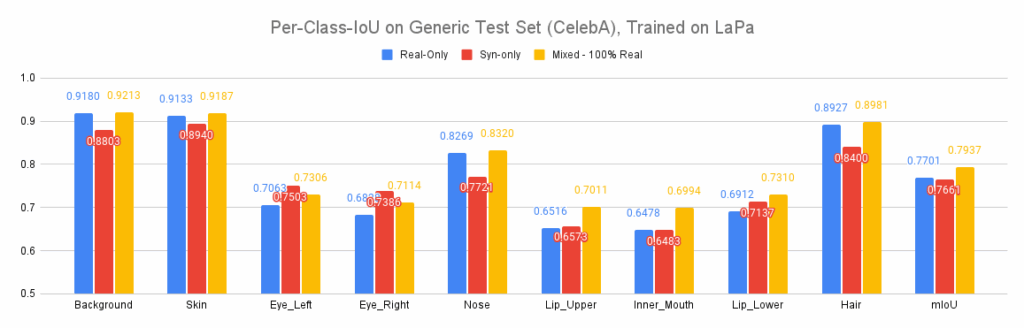
During cross-domain testing, synthetic data is competitive with real data and even outperforms it on difficult classes such as eyes and lips. Synthetic data seems to perform worse on nose and hair, but that can explained by differences in labelling of these two classes across real and synthetic.
Thus, in this very straightforward use case we have seen that even in a very direct application, with very efficient syn-to-real refinement, synthetic data generated by our Face API works basically at the same level as training on a different real dataset.
This is already very promising, but let us proceed to even more interesting use cases!
Background Matting: Synthetic Data for Very Complex Labeling
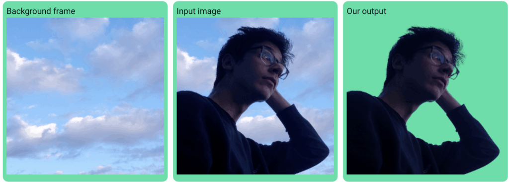
The primary use case for background matting, useful to keep in mind throughout this section, is cutting out a person from a “green screen” image/video or, even more interesting, from any background. This is, of course, a key computer vision problem in the current era of online videoconferencing.
Formally, background matting is a task very similar to face/person segmentation, but with two important differences. First, we are looking to predict not only the binary segmentation mask but also the alpha (opacity) value, so the result is a “soft” segmentation mask with values in the [0, 1] range. This is very important to improve blending into new backgrounds.
Second, the specific variation of background matting that we are experimenting with here takes two images as input: a pure background photo and a photo with the object (person). In other words, the matting problem here is to subtract the background from the foreground. Here is a sample image from the demo provided by Lin et al. (2020), the work that we take as the basic model for this study:
The purpose of this work was to speed up high-quality background matting for high-resolution images so that it could work in real time; indeed, Lin et al. have also developed a working Zoom plugin that works well in real videoconferencing.
We will not dwell on the model itself for too long. Basically, Lin et al. propose a pipeline that first produces a coarse output with atrous spatial pyramid pooling similar to DeepLabv3 (Chen et al., 2017) and then recover high-resolution matting details with a refinement network (not to be confused with syn-to-real refinement!). Here is the pipeline as illustrated in the paper:
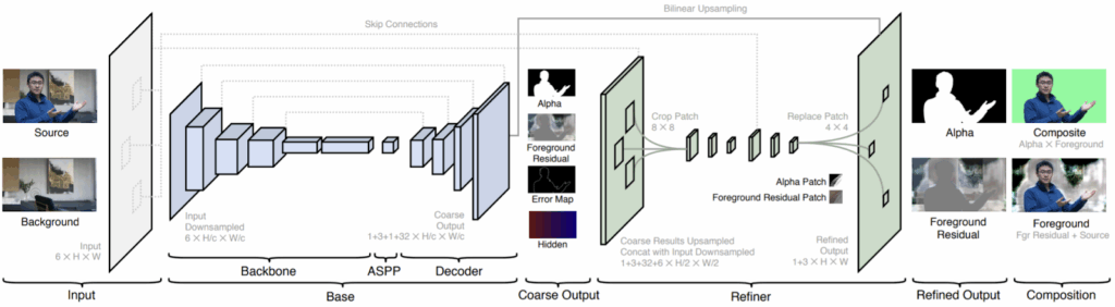
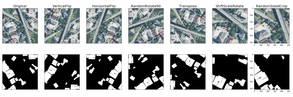
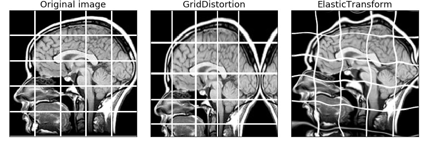
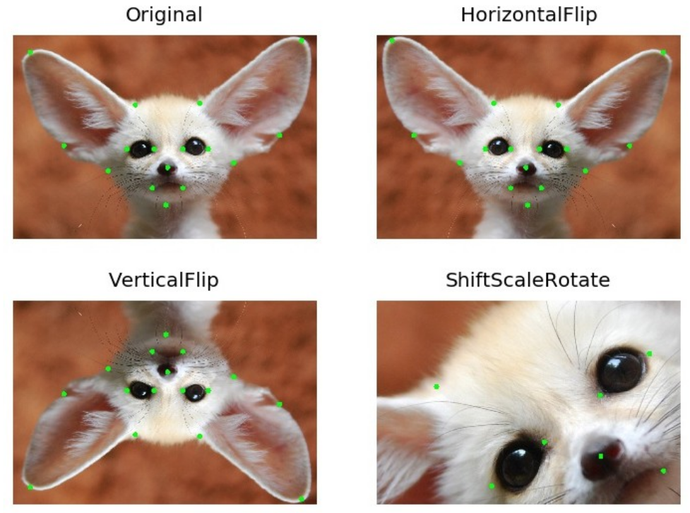
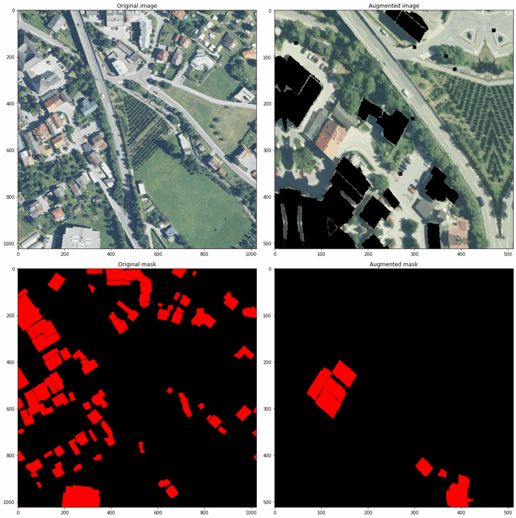
For our experiments, we have used the MobileNetV2 backbone (Sandler et al., 2018). For training we used virtually all parameters as provided by Lin et al. (2020) except augmentation, which we have made more robust.
One obvious problem with background matting is that it is extremely difficult to obtain real training data. Lin et al. describe the PhotoMatte13K dataset of 13,665 2304×3456 images with manually corrected mattes that they acquired, but release only the test set (85 images). Therefore, for real training we used the AISegment.com Human Matting Dataset (released on Kaggle) for the foreground part, refining its mattes a little with open source matting software (see below in more detail about this). The AISegment.com dataset contains ~30,000 600×800 images—note the huge difference in resolution with PhotoMatte13K.
Note that this dataset does not contain the corresponding background images, so for background images we used our own high-quality HDRI panoramas. In general, our pipeline for producing the real training set was as follows:
- cut out the object from an AISegment.com image according to the ground truth matte;
- take a background image, apply several relighting/distortion augmentations, and paste the object onto the resulting background image.
This is a standard way to obtain training sets for this problem. The currently largest academic dataset for this problem, Deep Image Matting by Xu et al. (2017), uses the same kind of procedure.
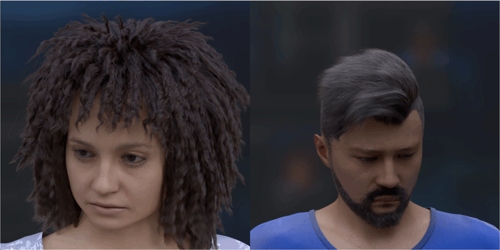
For the synthetic part, we used our Face API engine to generate a dataset of ~10K 1024×1024 images, using the same high-quality HDRI panoramas for the background. Naturally, the synthetic dataset has very accurate alpha channels, something that could hardly be achieved in manual labeling of real photographs. In the example below, note how hard it would be to label the hair for matting:
Before we proceed to the results, a couple of words about the quality metrics. We used slightly modified metrics from the original paper, also described in more detailed and motivated by Rhemann et al. (2009):
- mse: mean squared error for the alpha channel and foreground computed along the object boundary;
- mae: mean absolute error for the alpha channel and foreground computed along the object boundary;
- grad: spatial-gradient metric that measures the difference between the gradients of the computed alpha matte and the ground truth computed along the object boundary;
- conn: connectivity metric that measures average degrees of connectivity for individual pixels in the computed alpha matte and the ground truth computed along the object boundary;
- IOU: standard intersection over union metric for the “person” class segmentation obtained from the alpha matte by thresholding.
We have trained four models:
- Real model trained only on the real dataset;
- Synthetic model trained only on the synthetic dataset;
- Mixed model trained on a hybrid syn+real dataset;
- DA model, also trained on the hybrid syn+real dataset but with batchnorm-based domain adaptation as shown above updating batchnorm statistics only on the real training set.
The plots below show the quality metrics on the test set PhotoMatte85 (85 test images) where we used our HDRI panoramas as background images:
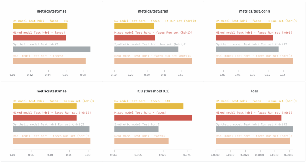
And here are the same metrics on the PhotoMatte85 test set with 4K images downloaded from the Web as background images:
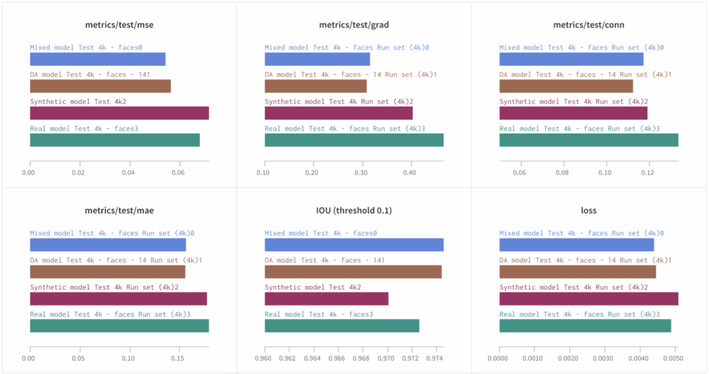
It is hard to give specific examples where the difference would be striking, but as you can see, adding even a small high-quality synthetic dataset (our synthetic set was ~3x smaller than the real dataset) brings tangible improvements in the quality. Moreover, for some metrics related to visual quality (conn and grad in particular) the model trained only on synthetic data shows better performance than the model trained on real data. The Mixed and DA models are better yet, and show improvements across all metrics, again demonstrating the power of mixed syn+real datasets.
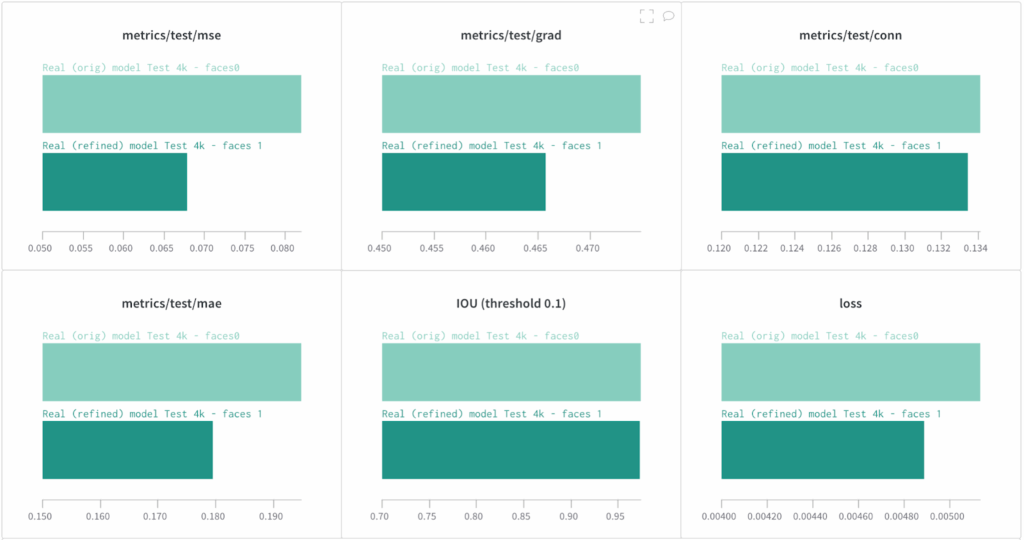
Above, we have mentioned automatic refinement of the AISegment.com dataset with open-source matting software that we applied before training. To confirm that these refinements indeed make the dataset better, we have compared the performance on refined and original AISegment.com dataset. The results clearly show that our refinement techniques bring important improvements:
Overall, in this case study we have seen how synthetic data helps in cases when real labeled data is very hard to come by. The next study is also related to human faces but switches from variants of segmentation to a slightly different problem.
Facial Landmark Detection: Fine-Tuning Beats Domain Adaptation
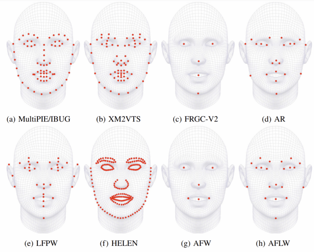
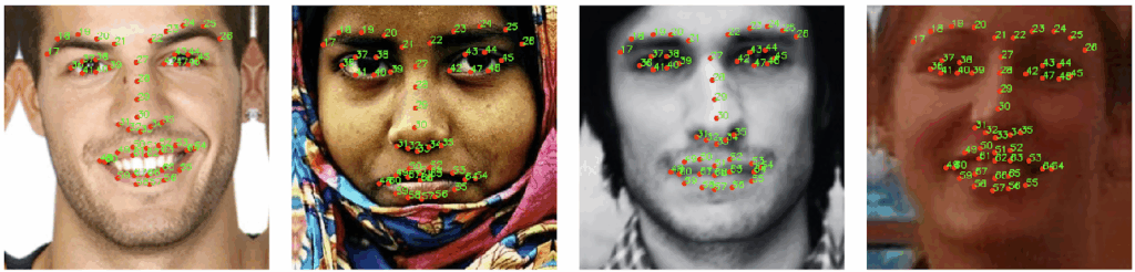
For many facial analysis tasks, including face recognition, face frontalization, and face 3D modeling, one of the key steps is facial landmark detection, which aims to locate some predefined keypoints on facial components. In particular, in this case study we used 51 out of 68 IBUG facial landmarks. Note that there are several different standards of facial landmarks, as illustrated below (Sagonas et al., 2016):
While this is a classic computer vision task with a long history, it unfortunately still suffers from many challenges in reality. In particular, many existing approaches struggle to cope with occlusions, extreme poses, difficult lighting conditions, and other problems. The occlusion problem is probably the most important obstacle to locating facial landmarks accurately.
As the basic model for recognizing facial landmarks, we use the stacked hourglass networks introduced by Newell et al. (2016). The architecture consists of multiple hourglass modules, each representing a fully convolutional encoder-decoder architecture with skip connections:
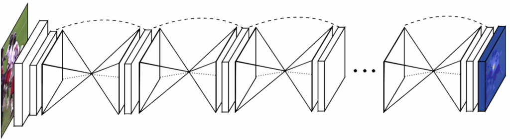
Again, we do not go into full details regarding the architecture and training process because we have not changed the basic model, our emphasis is on its performance across different training sets.
The test set in this study consists of real images and comes from the 300 Faces In-the-Wild (300W) Challenge (Sagonas et al., 2016). It consists of 300 indoor and 300 outdoor images of varying sizes that have ground truth manual labels. Here is a sample:
The real training set is a combination of several real datasets, semi-automatically unified to conform to the IBUG format. In total, we use ~3000 real images of varying sizes in the real training set.
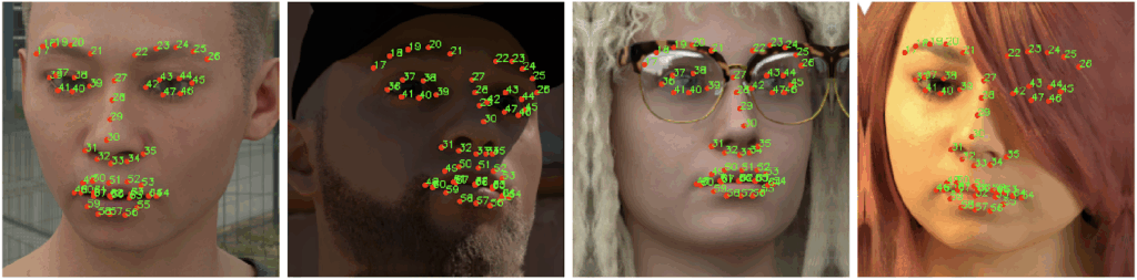
For the synthetic training set, since real train and test sets mostly contain frontal or near-frontal good quality images, we generated a relatively restricted dataset with the Face API, without images in extreme conditions but with some added racial diversity, mild variety in camera angles, and accessories. The main features of our synthetic training set are:
- 10,000 synthetic images with 1024×1024 resolution, with randomized facial attributes and uniformly represented ethnicities;
- 10% of the images contain (clear) glasses;
- 60% of the faces have a random expression (emotion) with intensity [0.7, 1.0], and 20% of the faces have a random expression with intensity [0.1, 0.3];
- the maximum angle of face to camera is 45 degrees; camera position and face angles are selected accordingly.
Here are some sample images from our synthetic training set:
Next we present our key results that were achieved with the synthetic training data in several different attempts at closing the domain gap. We present a comparison between 5 different setups:
- trained on real data only;
- trained on synthetic data only;
- trained on a mixture of synthetic and real datasets;
- trained on a mixture of synthetic and real datasets with domain adaptation based on batchnorm statistics;
- pretrained on the synthetic dataset and fine-tuned on real data.
We measure two standard metrics on the 300W test set: normalized mean error (NME), the normalized average Euclidean distance between true and predicted landmarks (smaller is better), and probability of correct keypoint (PCK), the percentage of detections that fall into a predefined range of normalized deviations (larger is better).
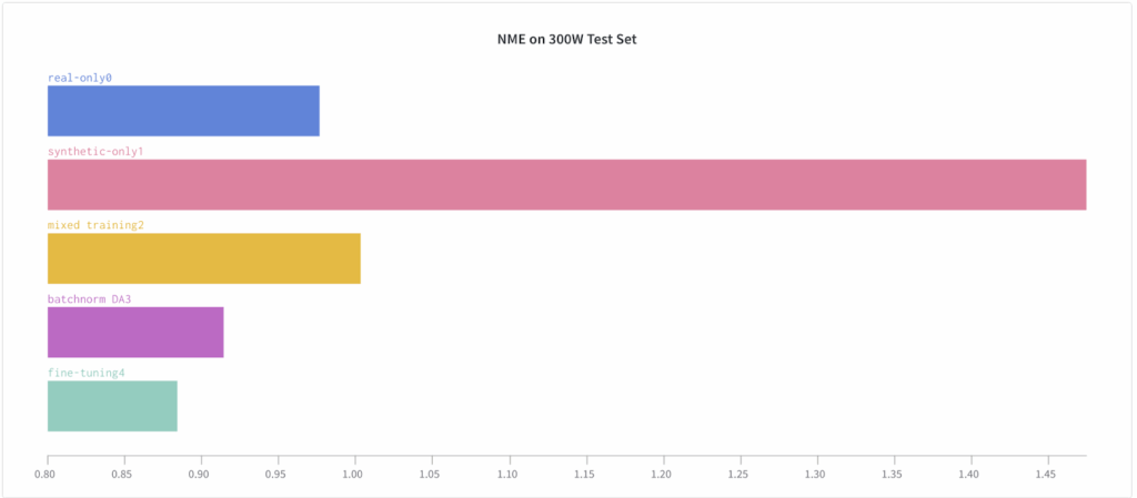
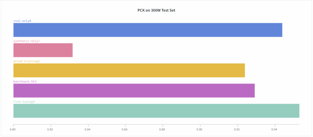
The results clearly show that while it is quite hard to outperform the real-only benchmark (the real training set is large and labeled well, and the models are well-tuned to this kind of data), facial landmark detection can still benefit significantly from a proper introduction of synthetic data.
Even more interestingly, we see that the improvement comes not from simply training on a hybrid dataset but from pretraining on a synthetic dataset and fine-tuning on real data.
To further investigate this effect, we have tested the fine-tuning approach across a variety of real dataset subsets. The plots below show that as the size of the real dataset used for fine-tuning decreases, the results also deteriorate (this is natural and expected):
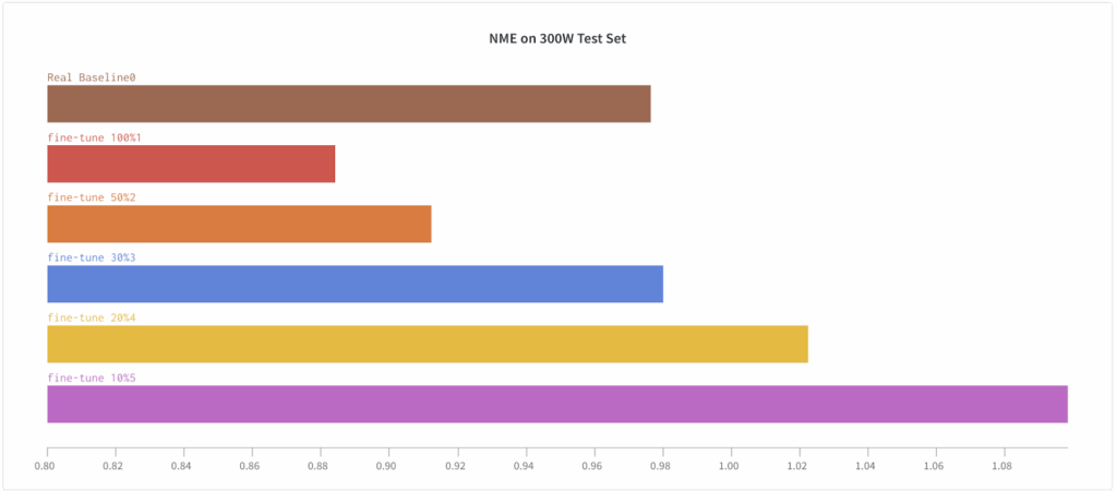
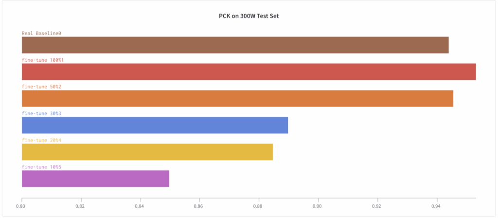
This fine-tuning approach is a training schedule that we have not often seen in literature, but here it proves to be a crucial component for success. Note that in the previous case study (background matting), we also tested this approach but it did not yield noticeable improvements.
Conclusion
In this whitepaper, we have considered simple ways to bring synthetic data into your computer vision projects. We have conducted three case studies for three different computer vision tasks related to human faces, using the power of Synthesis AI’s Face API to produce perfectly labeled and highly varied synthetic datasets. Let us draw some general conclusions from our results.
First of all, as the title suggests, it just works! In all case studies, we have been able to achieve significant improvements or results on par with real data by using synthetically generated datasets, without complex domain adaptation models. Our results suggest that synthetic data is a simple but very efficient way to improve computer vision models, especially in tasks with complex labeling.
Second, we have seen that synthetic-to-real domain gap can be the same as real-to-real domain gap. This is an interesting result because it suggests that while domain transfer still, obviously, remains a problem, it is not specific to synthetic data, which proves to be on par with real data if you train and test in different conditions. We have supported this with our face segmentation study.
Third, even a small amount of synthetic data can help a lot. This is a somewhat counterintuitive conclusion: traditionally, synthetic datasets have been all about quantity and diversity over quality. However, we have found that in problems where labels are very hard to come by and are often imprecise, such as background matting in one of our case studies, even a relatively small synthetic dataset can go a long way towards getting the labels correct for the model.
Fourth, fine-tuning on real data after pretraining on a synthetic dataset seems to work better than training on a hybrid dataset. We do not claim that this will always be the case, but a common theme in our case studies is that these approaches may indeed yield different results, and it might pay to investigate both (especially since they are very straightforward to implement and compare).
We believe that synthetic data may become one of the main driving forces for computer vision in the near future, as real datasets reach saturation and/or become hopelessly expensive. In this whitepaper, we have seen that it does not have to be hard to incorporate synthetic data into your models. Try it, it might just work!
Sergey Nikolenko
Head of AI, Synthesis AI

![\[\min_{\theta_G,\theta_T}\;\max_{\phi}\;\lambda_{1}\,\mathcal{L}_{\text{dom}}^{\text{PIX}}(D^{\text{PIX}},G^{\text{PIX}})+\lambda_{2}\,\mathcal{L}_{\text{task}}^{\text{PIX}}(G^{\text{PIX}},T^{\text{PIX}})+\lambda_{3}\,\mathcal{L}_{\text{cont}}^{\text{PIX}}(G^{\text{PIX}}),\]](https://blog.sergeynikolenko.ru/wp-content/ql-cache/quicklatex.com-957dcb2f206295ade0efd10261988ed3_l3.svg "Rendered by QuickLaTeX.com")
![\begin{align*}\mathcal{L}_{\text{dom}}^{\text{PIX}}(D^{\text{PIX}},G^{\text{PIX}}) =&\mathbb{E}_{\mathbf{x}_{S}\sim p_{\text{syn}}}\!\bigl[\log\!\bigl(1-D^{\text{PIX}}\!\bigl(G^{\text{PIX}}(\mathbf{x}_{S};\theta_{G});\phi\bigr)\bigr)\bigr]\\ +&\mathbb{E}_{\mathbf{x}_{T}\sim p_{\text{real}}}\!\bigl[\log D^{\text{PIX}}(\mathbf{x}_{T};\phi)\bigr];\end{align*}](https://blog.sergeynikolenko.ru/wp-content/ql-cache/quicklatex.com-efef45d7c7e94718bc3c779ccbd18aa7_l3.svg "Rendered by QuickLaTeX.com")
![\begin{align*}\mathcal{L}_{\text{task}}^{\text{PIX}}&(G^{\text{PIX}},T^{\text{PIX}}) = \\ &\mathbb{E}_{\mathbf{x}_{S},\mathbf{y}_{S}\sim p_{\text{syn}}} \!\bigl[-\mathbf{y}_{S}^{\top}\!\log T^{\text{PIX}}\!\bigl(G^{\text{PIX}}(\mathbf{x}_{S};\theta_{G});\theta_{T}\bigr) -\mathbf{y}_{S}^{\top}\!\log T^{\text{PIX}}(\mathbf{x}_{S};\theta_{T})\bigr],\end{align*}](https://blog.sergeynikolenko.ru/wp-content/ql-cache/quicklatex.com-b6a76786421e6e623da00bc4631f9bda_l3.svg "Rendered by QuickLaTeX.com")
![\begin{align*}\mathcal{L}_{\text{cont}}^{\text{PIX}}(G^{\text{PIX}}) =\mathbb{E}_{\mathbf{x}_{S}\sim p_{\text{syn}}}\!\Bigl[& \frac{1}{k}\,\lVert(\mathbf{x}_{S}-G^{\text{PIX}}(\mathbf{x}_{S};\theta_{G}))\odot m(\mathbf{x})\rVert_{2}^{2}\\ &-\frac{1}{k^{2}}\bigl((\mathbf{x}_{S}-G^{\text{PIX}}(\mathbf{x}_{S};\theta_{G}))^{\top}m(\mathbf{x})\bigr)^{2} \Bigr],\end{align*}](https://blog.sergeynikolenko.ru/wp-content/ql-cache/quicklatex.com-9b49079973db116b7c3f74dc0090161b_l3.svg "Rendered by QuickLaTeX.com")
 is a segmentation mask for the foreground object extracted from the synthetic data renderer; note that this loss does not “insist” on preserving pixel values in the object but rather encourages the model to change object pixels in a consistent way, preserving their pairwise differences.

![\[\mathcal{L}^{T2}=\mathcal{L}_{\text{GAN}}^{T2}(G_{S}^{T2},D_{T}^{T2})+\lambda_{1}\mathcal{L}_{\text{GAN}_f}^{T2}(f_{\text{task}}^{T2},D_{f}^{T2})+\lambda_{2}\mathcal{L}_{r}^{T2}(G_{S}^{T2})+\lambda_{3}\mathcal{L}_{t}^{T2}(f_{\text{task}}^{T2})+\lambda_{4}\mathcal{L}_{s}^{T2}(f_{\text{task}}^{T2}),\]](https://blog.sergeynikolenko.ru/wp-content/ql-cache/quicklatex.com-0993df42fb2d0258cab8f36cab798906_l3.svg "Rendered by QuickLaTeX.com")
![\begin{align*}\mathcal{L}_{\text{GAN}}^{T2}(G_{S}^{T2},D_{T}^{T2}) =&\mathbb{E}_{\mathbf{x}_{S}\sim p_{\text{syn}}} \bigl[\log(1-D_{T}^{T2}(G_{S}^{T2}(\mathbf{x}_{S})))\bigr]\\ +&\mathbb{E}_{\mathbf{x}_{T}\sim p_{\text{real}}} \bigl[\log D_{T}^{T2}(\mathbf{x}_{T})\bigr];\end{align*}](https://blog.sergeynikolenko.ru/wp-content/ql-cache/quicklatex.com-1633b4a1cb54b96701fbe567dda9832b_l3.svg "Rendered by QuickLaTeX.com")
![\begin{align*}\mathcal{L}_{\text{GAN}_f}^{T2}(f_{\text{task}}^{T2},D_{f}^{T2}) &=\mathbb{E}_{\mathbf{x}_{S}\sim p_{\text{syn}}} \bigl[\log D_{f}^{T2}(f_{\text{task}}^{T2}(G_{S}^{T2}(\mathbf{x}_{S})))\bigr]\\ &+\mathbb{E}_{\mathbf{x}_{T}\sim p_{\text{real}}} \bigl[\log(1-D_{f}^{T2}(f_{\text{task}}^{T2}(\mathbf{x}_{T})))\bigr]; \end{align*}](https://blog.sergeynikolenko.ru/wp-content/ql-cache/quicklatex.com-3df7b15dd51e4530b11b26b512dcab70_l3.svg "Rendered by QuickLaTeX.com")
 is the reconstruction loss for real images, simply an
  norm that says that T2Net is not supposed to change real images at all;
 is the task loss for depth estimation on synthetic images, namely the
  is the task loss for depth estimation on real images:
![\[\mathcal{L}_{s}^{T2}(f_{\text{task}}^{T2}) = |\partial_{x} f_{\text{task}}^{T2}(\mathbf{x}_{T})|^{-|\partial_{x}\mathbf{x}_{T}|} + |\partial_{y} f_{\text{task}}^{T2}(\mathbf{x}_{T})|^{-|\partial_{y}\mathbf{x}_{T}|},\]](https://blog.sergeynikolenko.ru/wp-content/ql-cache/quicklatex.com-6beff73b968312ed5f48a71d5509cc02_l3.svg "Rendered by QuickLaTeX.com")


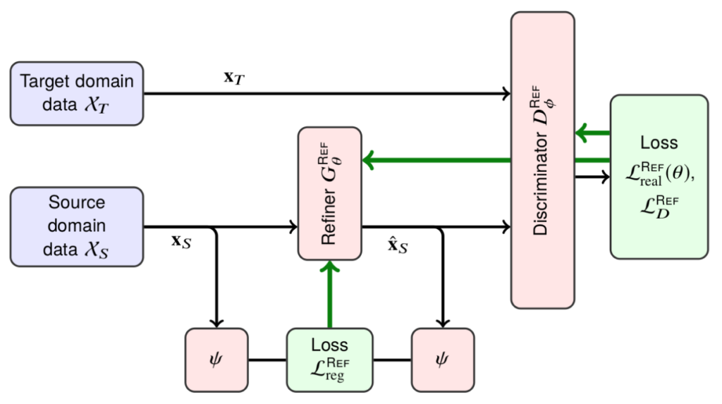
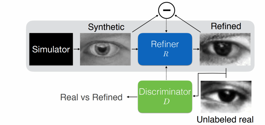
![\begin{align*}\mathcal{L}^{\text{REF}}_{G}(\theta) &= \mathbb{E}_{S}\Bigl[ \mathcal{L}^{\text{REF}}_{\text{real}}\!\bigl(\theta;\mathbf{x}_{S}\bigr) + \lambda\, \mathcal{L}^{\text{REF}}_{\text{reg}}\!\bigl(\theta;\mathbf{x}_{S}\bigr) \Bigr], \quad\text{where} \\[6pt]\mathcal{L}^{\text{REF}}_{\text{real}}\!\bigl(\theta;\mathbf{x}_{S}\bigr) &= -\,\log\!\Bigl(1 - D^{\text{REF}}_{\phi}\bigl(G^{\text{REF}}_{\theta}(\mathbf{x}_{S})\bigr)\Bigr), \\[6pt]\mathcal{L}^{\text{REF}}_{\text{reg}}\!\bigl(\theta;\mathbf{x}_{S}\bigr) &= \bigl\lVert \psi\!\bigl(G^{\text{REF}}_{\theta}(\mathbf{x}_{S})\bigr) - \psi(\mathbf{x}_{S}) \bigr\rVert_{1}\;.\end{align*}](https://blog.sergeynikolenko.ru/wp-content/ql-cache/quicklatex.com-5377b2ebb38f4ac4573f3e99f49cf12b_l3.svg "Rendered by QuickLaTeX.com")
 is a mapping into some kind of feature space. The feature space can contain the image itself, image derivatives, statistics of color channels, or features produced by a fixed extractor such as a pretrained CNN. But in case of SimGAN it was… in most cases, just an identity map. That is, the regularization loss simply told the generator to change as little as possible while still making the image realistic.
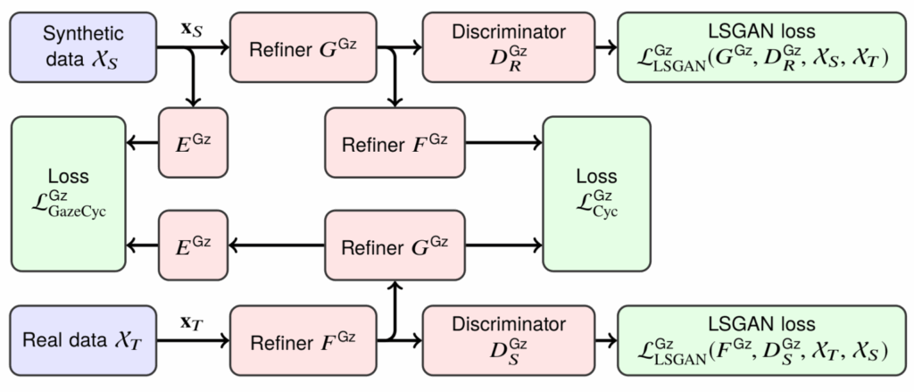
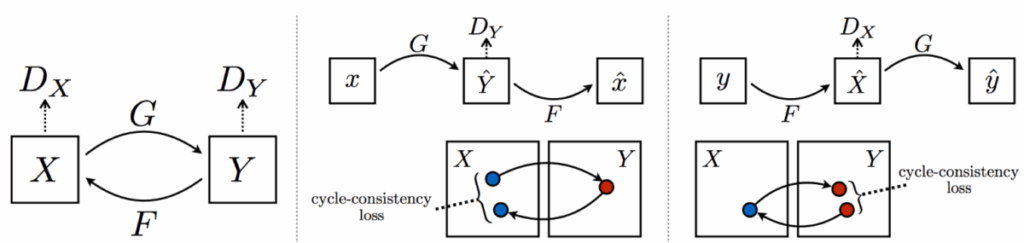
 and
and  , and two discriminators, one for the source domain and one for the target domain. What’s going on here?
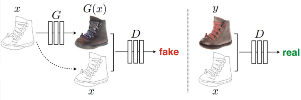

 can be a simple
  or
or 
![\begin{align*}\mathcal{L}_{\text{Cyc}}^{Gz}\!\bigl(G^{Gz},F^{Gz}\bigr) =& \mathbb{E}_{\mathbf{x}_{S}\sim p_{\text{syn}}} \!\Bigl[\bigl\|F^{Gz}\!\bigl(G^{Gz}(\mathbf{x}_{S})\bigr)-\mathbf{x}_{S}\bigr\|_{1}\Bigr]\\ +&\mathbb{E}_{\mathbf{x}_{T}\sim p_{\text{real}}} \!\Bigl[\bigl\|G^{Gz}\!\bigl(F^{Gz}(\mathbf{x}_{T})\bigr)-\mathbf{x}_{T}\bigr\|_{1}\Bigr];\end{align*}](https://blog.sergeynikolenko.ru/wp-content/ql-cache/quicklatex.com-a6479de0e633a11dae48f110a0f75e2b_l3.svg "Rendered by QuickLaTeX.com")
![\[\mathcal{L}_{\text{GazeCyc}}^{Gz}\bigl(G^{Gz},F^{Gz}\bigr) = \mathbb{E}_{\mathbf{x}_S\sim p_{\text{syn}}}\left[\left\| E^{Gz}\left(F^{Gz}(G^{Gz}(\mathbf{x}_S))\right) - E^{Gz}(\mathbf{x}_S)\right\|_2^2\right].\]](https://blog.sergeynikolenko.ru/wp-content/ql-cache/quicklatex.com-7ec6f9195cd5251a6e1ddcd68cabef95_l3.svg "Rendered by QuickLaTeX.com")
![\begin{align*}\min_{D}\; V_{\text{LSGAN}}(D)&= \tfrac12\,\mathbb{E}_{\mathbf{x}\sim p{\text{data}}}\bigl[(D(\mathbf{x}) - b)^{2}\bigr]+ \tfrac12\,\mathbb{E}_{\mathbf{z}\sim p{z}}\bigl[(D(G(\mathbf{z})) - a)^{2}\bigr], \\\min_{G}\; V_{\text{LSGAN}}(G)&= \tfrac12\,\mathbb{E}_{\mathbf{z}\sim p{z}}\bigl[(D(G(\mathbf{z})) - c)^{2}\bigr],\end{align*}](https://blog.sergeynikolenko.ru/wp-content/ql-cache/quicklatex.com-17085664f89788591d5bd50a9582c94f_l3.svg "Rendered by QuickLaTeX.com")
 on real images and some other constant
  on fake images, while the generator is trying to convince the discriminator to output c on fake images (it has no control over the real ones). Naturally, usually one takes
  and
and  , although there is an interesting theoretical result about the case when
  and
and  , that is, when the generator is trying to make the discriminator maximally unsure about the fake images.
![\[\mathcal{L}_{\text{LSGAN}}^{Gz}(G, D, S, R) = \mathbb{E}_{\mathbf{x}_S \sim p{_\text{syn}}}\Bigl[\,\bigl(D\bigl(G(\mathbf{x}_S)\bigr) - 0.9\bigr)^{2}\Bigr] + \mathbb{E}_{\mathbf{x}_T \sim p_{\text{real}}}\Bigl[\,D(\mathbf{x}_T)^{2}\Bigr];\]](https://blog.sergeynikolenko.ru/wp-content/ql-cache/quicklatex.com-2c73a446a0e5b4c80b7031df6b98840f_l3.svg "Rendered by QuickLaTeX.com")


![\begin{align*}\tilde{x} &= \lambda x_i + (1 - \lambda) x_j,&\text{where } x_i, x_j \text{ are raw input vectors,} \\[4pt]\tilde{y} &= \lambda y_i + (1 - \lambda) y_j,&\text{where } y_i, y_j \text{ are one-hot label encodings.}\end{align*}](https://blog.sergeynikolenko.ru/wp-content/ql-cache/quicklatex.com-dc7c242c1407bae338fe0bb1b9014ef1_l3.svg "Rendered by QuickLaTeX.com")