Last time, we finished all intended mathematical content, so it is time for us to wrap up the generative AI series. We will do it over two installments. Today, we discuss and summarize the (lots of) news that have been happening in the AI space over the last half a year. They all conveniently fall into the generative AI space, with expanding capabilities leading to both extreme excitement and serious security concerns. So how are current AI models different from older ones and when are we going to actually have AGI? It all started with GPT-3.5…

Large Language Models: I Heard You Like Hype Waves
Artificial intelligence has a history of ups and downs. The initial wave of excitement after the 1956 Dartmouth seminar ended with the “AI winter” that spanned the 1970s and early 1980s. Then people realized that they could train deep neural networks, and hopes were again high, but it again turned out to be a false start mostly due to insufficient computing power (image source):
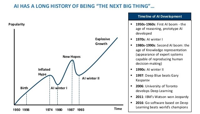
Finally, in the mid-2000s deep learning started to work in earnest, and we have been living on another hype wave of artificial intelligence ever since. The first transformative real world application was in speech recognition and processing (voice assistants were made possible by early deep neural networks), then AlexNet revolutionized image processing, then deep neural networks came into natural language processing, and so on, and so forth.
But you can have hype waves inside hype waves. And this is exactly what has been happening with large language models over the last year or so, especially last spring. By now, researchers are seriously considering the possibility that we can reach AGI (artificial general intelligence, usually taken to mean human-level or stronger) with our current basic approach, maybe just by scaling it up and thinking of a few more nice tricks for training it.
How did that happen? Let’s first understand what we are talking about.
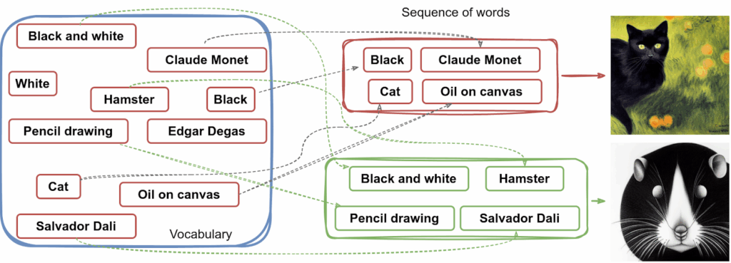
A language model is a machine learning model that predicts the next token in a sequence of language tokens; it’s easier to think of tokens as words, although in reality models usually break words down into smaller chunks. The machine learning problem here is basically classification: what’s the next token going to be?
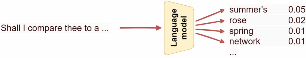
By continuously predicting the next token, a language model can write text, and the better the language model, the more coherent the resulting text can be:
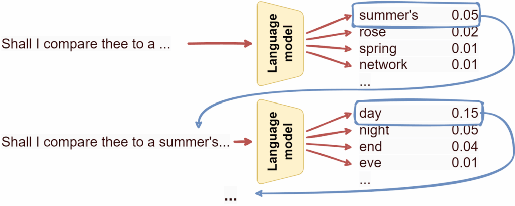
Note that that’s the only thing a language model can do: predict the next token, over and over.
Language models appeared a very long time ago. In fact, one of the first practical examples of a Markov chain, given by Andrei Markov himself in 1913, was a simple language model that learned how likely vowels and consonants are to follow each other in the Russian language.
Up until quite recently, language models were Markovian in nature, but the deep learning revolution changed that: recurrent networks were able to hold a consistent latent state and pass it through to the next time slot, which could improve token predictions. But the real game changer came with Transformers, attention-based architectures that started another hype wave on top of deep learning itself.
Just like deep neural networks were used to achieve state of the art results in virtually every field of machine learning in 2005-2020, after 2017-2018 Transformers did the same thing inside neural networks: the Transformer was invented as an encoder-decoder architecture for machine translation but soon branched into language modeling, general text understanding, and later image understanding, speech recognition, and many, many other fields, becoming a ubiquitous tool.
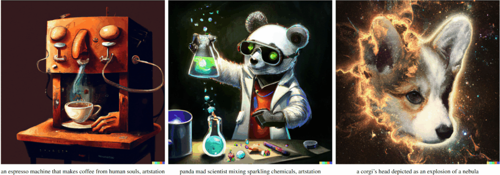
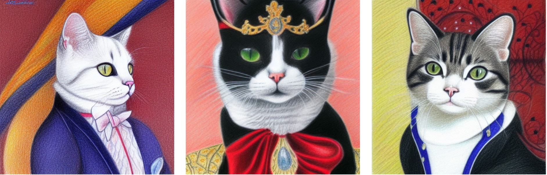
Still, there is another hype wave inside the Transformers that we are interested in today. So now we are talking about a wave on top of a wave on top of a wave… well, this is the best I could do with Stable Diffusion:
This latest craze started when OpenAI updated its GPT-3 model with fine-tuning techniques that used human feedback. Introduced in InstructGPT in the spring of 2022, these techniques allowed to make a pure token prediction machine more useful for human-initiated tasks by fine-tuning it on human assessments. An assessor labels how useful and/or harmless was the model’s reply, and the model learns to be more useful and less harmful (more on that later). In this way, a model can learn, for example, to answer human questions with answers that it “considers” to be correct, rather than just continue the conversation by changing the subject or asking a question itself (which could be a quite plausible hypothesis if we are just predicting the next token).
The fine-tuned models are known as the GPT-3.5 series, and the fine-tuning process itself was finally developed into reinforcement learning from human feedback (RLHF). With RLHF, GPT-3.5 turned into ChatGPT, the model you have definitely heard about. Starting from GPT-3, such models have become collectively known as large language models (LLM), a term basically meaning “large enough to be interesting in practice”. “Large enough” indeed proves to be quite large: GPT-3 (and hence ChatGPT) has about 175 billion trainable parameters.
Still, note that ChatGPT in essence is still a language model, that is, just a machine for predicting the next token in a text trained on enormous datasets that encompass the whole available Internet. Interestingly enough, that proves to be sufficient for many different applications.
The AI Spring of 2023
After ChatGPT was released in November 2022, it became the fastest growing app ever, and the user base grew exponentially. It took a record 5 days to get to 1 million users, and by now ChatGPT has over 100 million users, a number that has probably already more or less saturated but shows few signs of dropping.
We entered 2023 with ChatGPT, but it turned out to be only the beginning. Here is a timeline of just the main developments in this latest spring of AI:
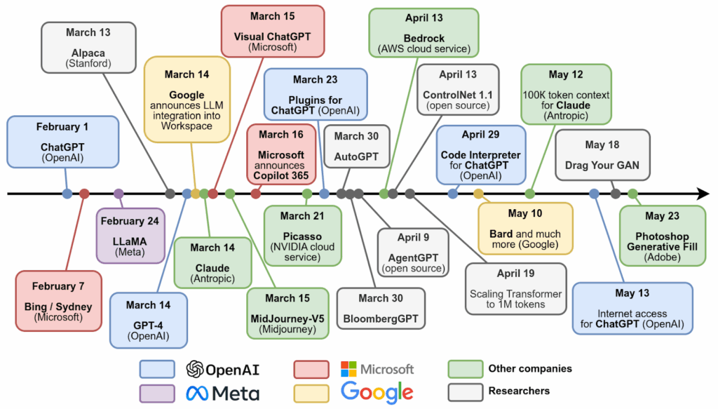
Let’s walk through some of them.
On February 7, Microsoft announced its own answer to ChatGPT, a language model that was supposed to help Bing search. This release proved to be a little premature: the model was quickly jailbroken by the users, revealed its internal name Sydney, and made some interesting comments about it (I did a rather sloppy censoring job below):

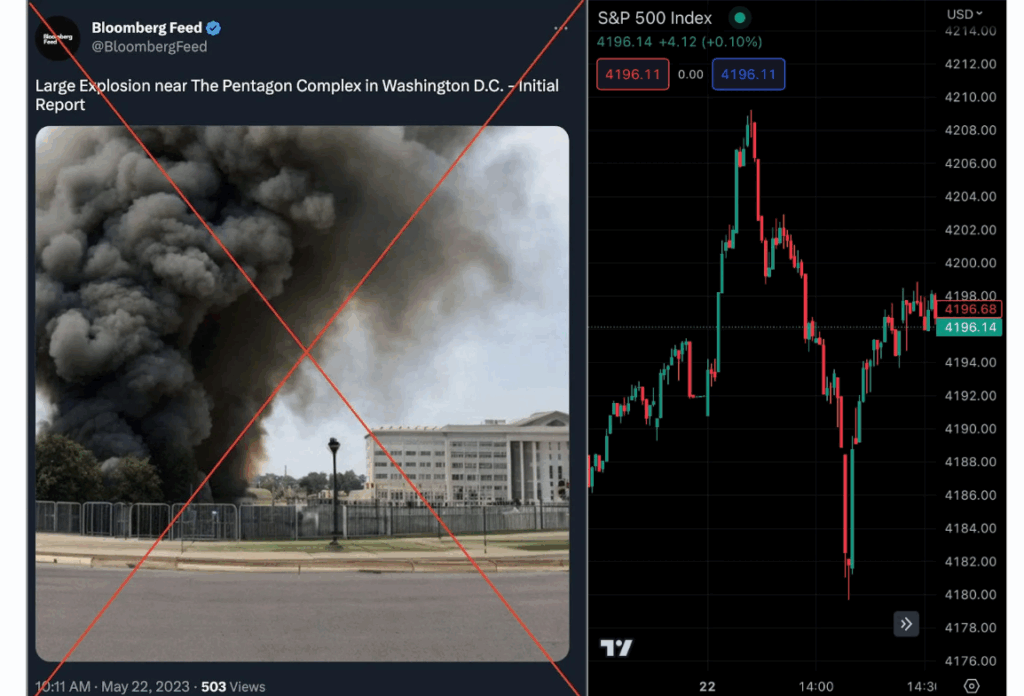
In a way, this is the first time it got into the public consciousness that even the current crop of LLMs may be somewhat dangerous. And yes, I’m still not quite used to this:

On February 24, Facebook AI Research (FAIR) released the LLaMA model (Large Language Model Meta AI). It’s questionable that LLaMA by itself is any better than GPT-3.5 but LLaMA is important because it is open source. Anyone can download the pretrained model weights, which opened up large language models for a huge community of enthusiasts: you cannot train a GPT-3 sized model at home but you sure can experiment with it, do prompt engineering, maybe even fine-tune it. LLaMA has already led to many new developments from independent researchers, and the recently released LLaMA 2 (July 2023) is sure to follow suit.
March 14 became the most important single day in this spring of AI. On the same day:
- Google announced that it would integrate large language models into its ecosystem (that is, Google Docs etc.),
- Antropic, a startup branched from OpenAI with a special interest in AI safety, released its first LLM called Claude,
- but OpenAI stole the day from those two by announcing its next level GPT-4 model.
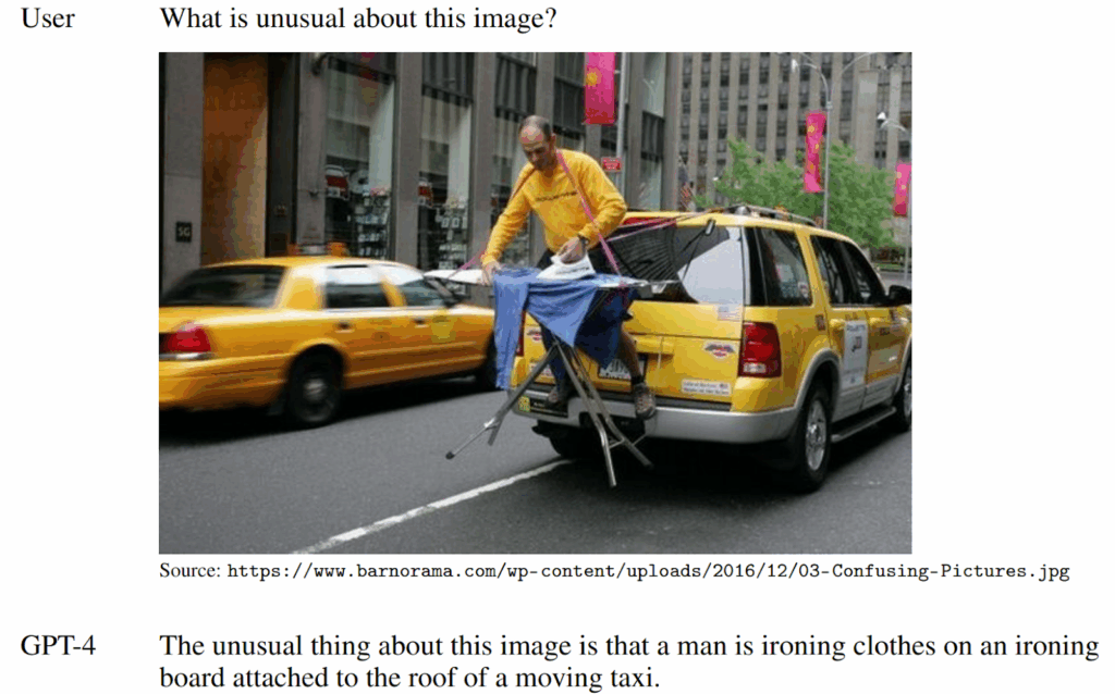
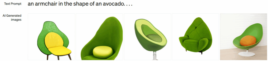
GPT-4 is supposed to be multimodal, that is, it is able to process both text and images at the same time. At the time of writing, its multimodal capabilities are not yet available to the general public, but existing illustrations from the papers are quite convincing. Here is an example from the original work:
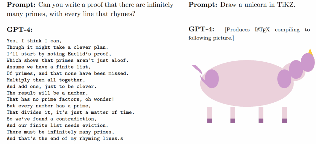
But to get a better grasp on GPT-4 capabilities, I really recommend reading the paper called “Sparks of Artificial General Intelligence: Early experiments with GPT-4”, also released in March. Their experimental results are eerily good even if cherry-picked:
Around the same time, OpenAI released a plugin mechanism that allowed people to build upon ChatGPT via prompt engineering, and In April serious projects of this kind started to appear. One of the most interesting such projects was AutoGPT, a plugin that tries (sometimes quite successfully) to make a language model into an agent that acts independently and intelligently to achieve its goals. AutoGPT was advertised as a personal AI assistant, able to achieve the goals set by a user via planning, setting and fulfilling subgoals, analyzing data found on the Web and on the user’s computer. Right now AutoGPT does not look very successful but it is an interesting attempt to make language models agentic (more on that later).
In May, Google released Bard that proved to be much more successful than Sydney, and made the support for LLMs in the Google ecosystem actually starting to happen. Research-wise, late April and May saw several interesting results aimed at extending the context window for LLMs, that is, how many tokens they can take in and process at a time. Here I will highlight the paper “Scaling Transformer to 1M tokens and beyond with RMT” and Antropic expanding Claude’s context window to 100K tokens. This is already hundreds of pages that a language model can process together, summarize, try to derive new insights, and so on.
In the last couple of months, this torrent of new AI capabilities has slowed down somewhat. But what does it actually mean? Are we going to have AGI soon? Will AI take our jobs? What’s the plan? Let’s see where we stand right now and what are the projections.
When AGI?
ChatGPT and GPT-4 can be transformative in their own right, but what about actual strong artificial intelligence (artificial general intelligence, AGI)? When are we going to have actual human-level intellect in AI models?
AI has a history of extra optimistic forecasts. For a long time, the AI optimists have been predicting true AGI being about 30 years from whenever the survey was held. That’s understandable: an AI guru would predict that he or she would live to see the true AGI, but in some distant future, not right now. Still, let’s see what the forecasters say now.
There are approaches to making AGI forecasts by continuing trend lines—naturally, the problem is which trend line to choose. For example, Ajeya Cotra (2020) tried to anchor AGI development in biological analogies. There are several ways to use biology as a measure of how much computation we need to get to human level:
- there are about 1015 parameters (synapses) in a human brain;
- to learn the weights for these synapses, we make about 1024 computations during our lifetimes;
- but to get to the human brain, evolution required about 1052 computations to create our genome (yes, you can have a ballpark estimate even for that).
The first estimate is clearly too low, the last one is clearly too high, so the truth must be somewhere in between… but where exactly, and why are we supposing that the human brain has any relevance at all? We were abstractly motivated by birds in our desire to fly but inventing the airplane had no relation to avian evolutionary development.
For a different example, Davidson (2021) constructed a model that can make predictions on AI development via what they call semi-informative priors. But if you look inside the model, all you see is a Markov chain of events like “we tried to develop AGI and failed, next year we tried twice”…
In my opinion, all we really have are still expert surveys. In August 2022, Grace, Weinstein-Raun, and Stein-Perlman conducted a survey of 738 AI experts (defined as people who authored papers on NeurIPS and ICML). Their median estimate was that we have a 50% chance to develop human-level intelligence in 37 years, by 2059; this is a very close match with the previous survey, conducted in 2016, that placed AGI in 2061.
Still, these are just medians of some very wide distributions. Wynroe et al. (2023) attempted a meta-review of various transformative AI timelines. Here are the cumulative distribution functions they had:
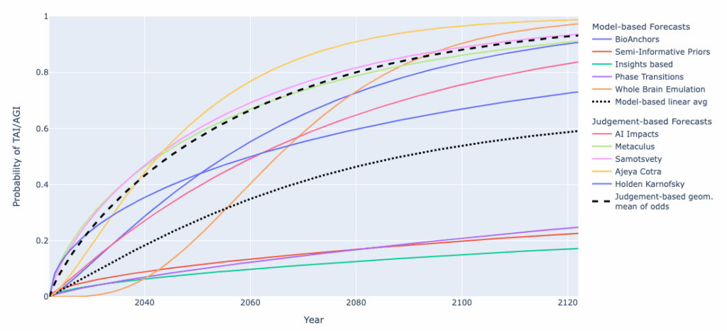
And if you prefer numbers, here is a summary table of various percentiles:
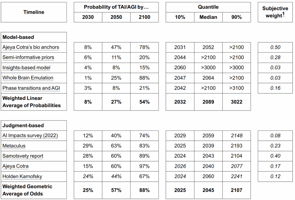
As you can see, experts believe there is a significant chance to achieve AGI by 2050 (more than half) and we are about 90% certain to get there by 2100. Model-based estimates are much more modest but here we average it with evolutionary bio-anchors and whole brain emulations that are hard to believe to be necessary. Still, all of these estimates have extremely wide margins: nobody knows if the path to AGI is already open (and it’s just a matter of scale and lots of compute) or if it requires more conceptual breakthroughs.
Finally, these days there are people who put their money where their mouths are. The Metaculus prediction market has a popular question that reads as follows: “When will the first general AI system be devised, tested, and publicly announced?” At present (Sep 18, 2023), the forecasting community has a median prediction of 2032:
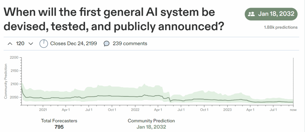
Interestingly, last time I checked (in July) their median was November 2032, so it’s slowly creeping up. However, since Metaculus handles real bets, they have to have specific resolution criteria for general AI. In this case, it’s a:
- two-hour adversarial Turing test,
- general robotic capabilities,
- and human-level or superhuman results on several general-purpose datasets (see the question page for details).
While this is as good a take on an instrumental definition of AGI as any, I can definitely foresee a model that does all that but is not considered “general AI”, just like many previous benchmarks have been overcome in the past.
So in summary, I would say that current forecasts are not that different from earlier AI history: we hope to see AGI during our lifetimes, we are far from sure we will, and it’s still hard to define what it is, even as we may be on the very brink of it.
How AGI? Slow vs. fast takeoff
Another interesting discussion is not about when AGI comes but about how it is going to happen. Back in 1965, Irving J. Good, a British mathematician and Turing’s coworker at Bletchley Park, suggested the idea of an “intelligence explosion”: a machine with superhuman intelligence will be able to design new intelligent machines faster than humans can, those machines will work faster yet, and ultimately the process will converge to physical limits, and progress will be faster than humans can even notice. This point, when progress becomes “infinitely” fast, is known as the technological singularity.
Technological singularity due to AGI sounds plausible to most thinkers, but opinions differ on how we get there. The current debate is between “slow takeoff” and “fast takeoff” models: how fast is AGI going to happen and are we going to get any warning about it?
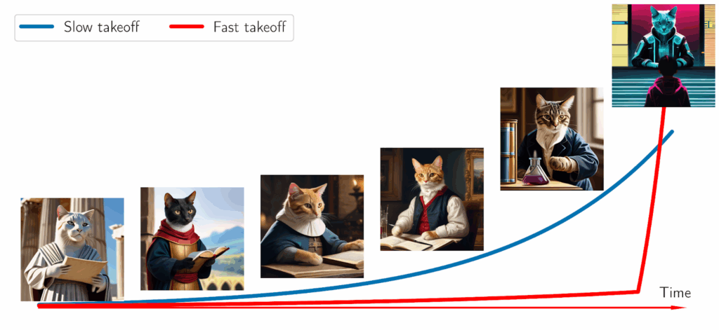
In the slow takeoff model, AI has a lot of impact on the world, this impact is very noticeable, and, for instance, the world GDP has an order of magnitude growth due to AI before we have the true AGI that could be dangerous. In this model, AI and even AGI falls into the regular technological progress trends and serves as an important but ultimately yet another technological revolution that will allow these trends to continue further. AI can speed up progress further but it’s just human progress continuing along its exponential trend lines.
In the fast takeoff scenario, AI can and will have an effect in line with “regular” technological progress, but that happens right until the singularity, and then it snowballs very quickly, too quickly for humans to do anything about it. The central scenario for fast takeoff goes as follows: after a certain threshold of capabilities, we get an AI that is simultaneously agentic (which in particular means that it wants power—we’ll get to it in the next post) and able to improve itself. After that, we don’t get any further warnings: the AI improves itself very quickly, quietly obtains sufficient resources, and then simply takes over.
There have been interesting debates about this that are worth reading. The main proponent of the fast takeoff scenario is Eliezer Yudkowsky, who has been warning us about potential AGI dangers for over a decade; we will consider his work in much more detail in the next post.
But it’s worth keeping in mind that slow takeoff is “slow” in the sense that we are going to notice. But even the slow takeoff scenario predicts exponential growth! It assumes only a couple of years or maybe even several months between the AI starting to visibly transform society and the arrival of real superhuman AGI. Fast takeoff says it might take seconds… but, to be honest, a year also does not sound like enough time to prepare unless we start now.
All of this means that we better be ready to face AGI in our lifetimes, perhaps unexpectedly and almost certainly with a very short development timescale. Are we?..
Conclusion
This is the last question still left for us in this series: are we ready for AGI?
Next time, we will discuss the dangers that potentially superhuman AI can pose for humanity. This includes the “mundane” dangers such as the loss of jobs due to this next round of the industrial revolution. But it also includes the potential existential risk of having an AGI that’s smarter than us, more powerful than us, but does not share our values and does not care about humans at all. We will see why it is reasonable to be afraid, what the hard problems are, and how we are currently trying to tackle them. In any case, we sure live in some very interesting times—let’s see what the future brings!
Sergey Nikolenko
Head of AI, Synthesis AI


 , where
  is the input image and
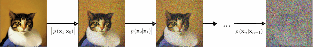
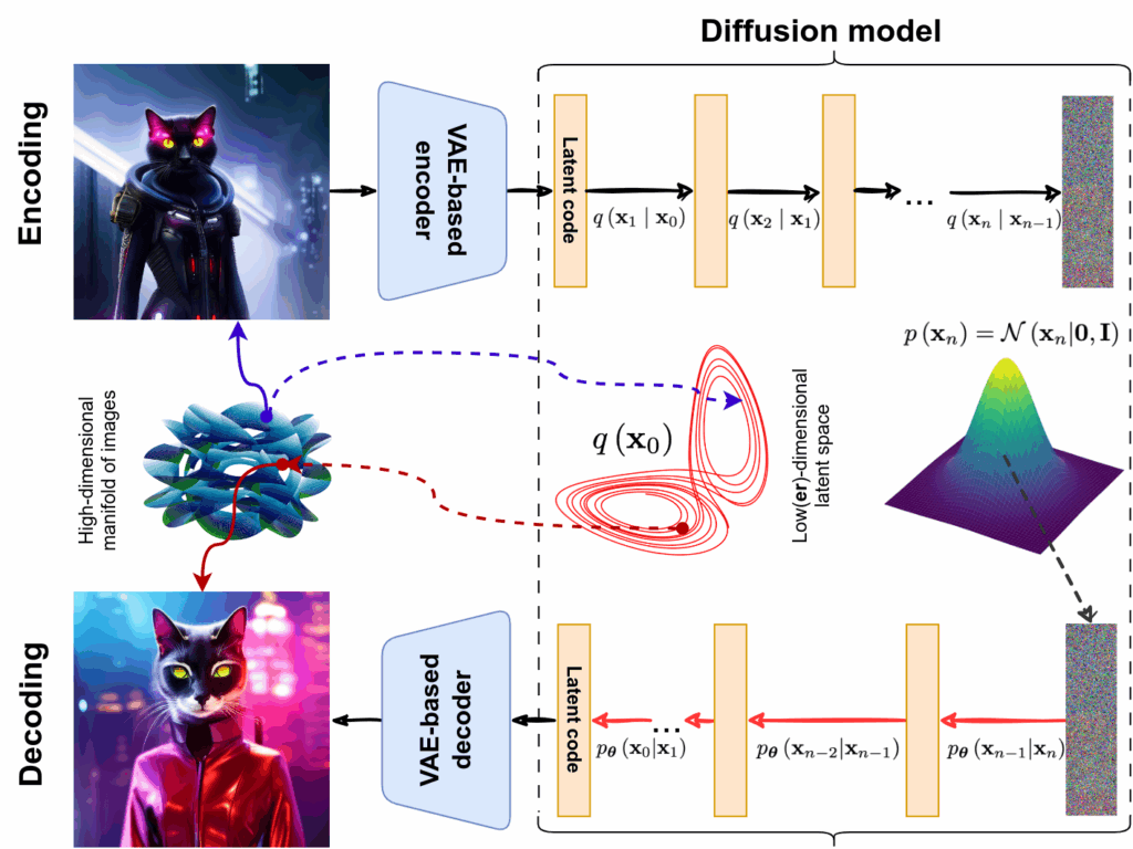
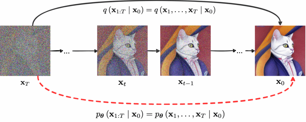
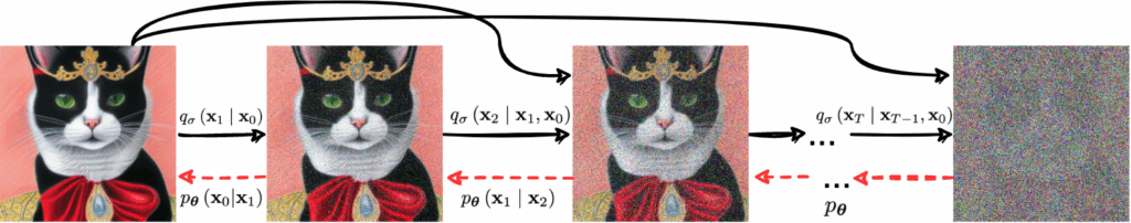
  is the image with added noise. Applying this distribution repeatedly, we get a Markov chain called forward diffusion that gradually adds noise until the image is completely unrecognizable:
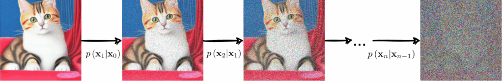
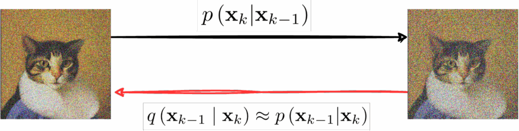
 with model parameters
  that should be a good approximation for the inverted
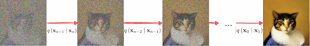
  , you can presumably run it backwards and get the images back from basically random noise. This process is known as reverse diffusion:
 to
to  . Since we already know
  is a Gaussian with variance
  and mean that reduces
  by a factor of the square root of
  (this is necessary to make the process variance preserving, so that
  would not explode or vanish), and the entire process takes T steps:
![\[q(\mathbf{x}_t | \mathbf{x}_{t-1}) = \mathcal{N}\left(\mathbf{x}_t | \sqrt{1-\beta_t}\mathbf{x}_{t-1}, \beta_t\mathbf{I}\right),\qquad q\left(\mathbf{x}_{1:T} | \mathbf{x}_0\right) = \prod_{t=1}^T q\left(\mathbf{x}_t | \mathbf{x}_{t-1}\right).\]](https://blog.sergeynikolenko.ru/wp-content/ql-cache/quicklatex.com-3f2b1e0a2aa9e1fc77fd89d9176d97ed_l3.svg "Rendered by QuickLaTeX.com")

 is also a Gaussian, and we know its parameters:
![\[q\left(\mathbf{x}_{t} | \mathbf{x}_0\right) = \mathcal{N}\left(\mathbf{x}_{t} | \sqrt{A_t}\mathbf{x}_0, \left(1-A_t\right)\mathbf{I}\right).\]](https://blog.sergeynikolenko.ru/wp-content/ql-cache/quicklatex.com-42a7387facdf0eee73c05da98615c98a_l3.svg "Rendered by QuickLaTeX.com")
 directly, in closed form, without having to go through any intermediate steps.
 , it would be easy! Let’s use the Bayes formula and substitute distributions that we already know:

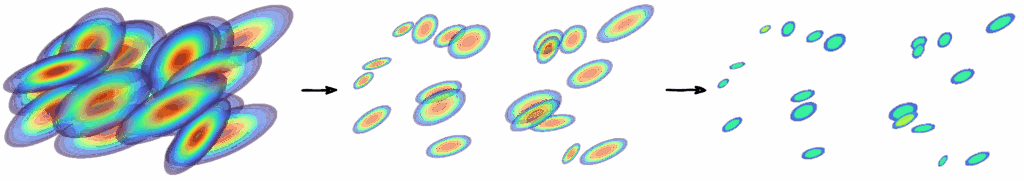
 that represents the impossibly messy distribution of, say, real life images. Ultimately we want our reverse diffusion process to reconstruct
  ; something like this:
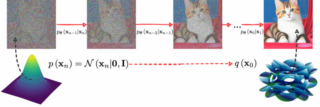
 , with no conditioning on the unknown
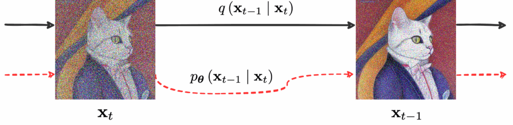
 :
:
![\[\log p_{\boldsymbol{\theta}}(\mathbf{x}_0) = \log p_{\boldsymbol{\theta}}(\mathbf{x}_0,\mathbf{x}_1,\ldots,\mathbf{x}_T) - \log p_{\boldsymbol{\theta}}(\mathbf{x}_1,\ldots,\mathbf{x}_T|\mathbf{x}_0),\]](https://blog.sergeynikolenko.ru/wp-content/ql-cache/quicklatex.com-9b929bc3f16ece335bb0fe3af038534e_l3.svg "Rendered by QuickLaTeX.com")
 , and then add and subtract
  on the right-hand side:
![\begin{align*}\mathbb{E}_{q(\mathbf{x}_{0})}\left[\log p_{\boldsymbol{\theta}}(\mathbf{x}_0)\right] &= \mathbb{E}_{q(\mathbf{x}_{0:T})}\left[\log p_{\boldsymbol{\theta}}(\mathbf{x}_{0:T})\right] - \mathbb{E}_{q(\mathbf{x}_{0:T})}\left[\log p_{\boldsymbol{\theta}}(\mathbf{x}_{1:T}|\mathbf{x}_0)\right] \\ & = \mathbb{E}_{q(\mathbf{x}_{0:T})}\left[\log\frac{p_{\boldsymbol{\theta}}(\mathbf{x}_{0:T})}{q(\mathbf{x}_{1:T}|\mathbf{x}_{0})}\right] + \mathbb{E}_{q(\mathbf{x}_{0:T})}\left[\log\frac{q(\mathbf{x}_{1:T}|\mathbf{x}_{0})}{p_{\boldsymbol{\theta}}(\mathbf{x}_{1:T}|\mathbf{x}_{0})}\right].\end{align*}](https://blog.sergeynikolenko.ru/wp-content/ql-cache/quicklatex.com-889edd5ef0cc407f9373b90208aad17c_l3.svg "Rendered by QuickLaTeX.com")
 and
and  , so that’s what we want to minimize in the approximation. Since on the left-hand side we have a constant independent of
  minimizing the KL divergence with respect to
 ![\begin{align*}\mathcal{L} =& \mathbb{E}_{q}\left[\log\frac{q(\mathbf{x}_{1:T}|\mathbf{x}_{0})}{p_{\boldsymbol{\theta}}(\mathbf{x}_{0:T})}\right] = \mathbb{E}_{q}\left[\log\frac{\prod_{t=1}^Tq(\mathbf{x}_{t}|\mathbf{x}_{t-1})}{p_{\boldsymbol{\theta}}(\mathbf{x}_{T})\prod_{t=1}^Tp_{\boldsymbol{\theta}}(\mathbf{x}_{t-1}|\mathbf{x}_{t})}\right] \\=& \mathbb{E}_{q}\left[-\log p_{\boldsymbol{\theta}}(\mathbf{x}_{T}) + \sum_{t=1}^T\log\frac{q(\mathbf{x}_{t}|\mathbf{x}_{t-1})}{p_{\boldsymbol{\theta}}(\mathbf{x}_{t-1}|\mathbf{x}_{t})}\right] \\=& \mathbb{E}_{q}\left[-\log p_{\boldsymbol{\theta}}(\mathbf{x}_{T}) + \sum_{t=2}^T\log\frac{q(\mathbf{x}_{t}|\mathbf{x}_{t-1})}{p_{\boldsymbol{\theta}}(\mathbf{x}_{t-1}|\mathbf{x}_{t})} + \log\frac{q(\mathbf{x}_{1}|\mathbf{x}_{0})}{p_{\boldsymbol{\theta}}(\mathbf{x}_{0}|\mathbf{x}_{1})}\right] \\=& \mathbb{E}_{q}\left[-\log p_{\boldsymbol{\theta}}(\mathbf{x}_{T}) + \sum_{t=2}^T\log\left(\frac{q(\mathbf{x}_{t}|\mathbf{x}_{t-1},\mathbf{x}_{0})}{p_{\boldsymbol{\theta}}(\mathbf{x}_{t-1}|\mathbf{x}_{t})}\frac{q(\mathbf{x}_{t}|\mathbf{x}_{0})}{q(\mathbf{x}_{t-1}|\mathbf{x}_{0})}\right) + \log\frac{q(\mathbf{x}_{1}|\mathbf{x}_{0})}{p_{\boldsymbol{\theta}}(\mathbf{x}_{0}|\mathbf{x}_{1})}\right] \\=& \mathbb{E}_{q}\left[-\log p_{\boldsymbol{\theta}}(\mathbf{x}_{T}) + \sum_{t=2}^T\log\frac{q(\mathbf{x}_{t}|\mathbf{x}_{t-1},\mathbf{x}_{0})}{p_{\boldsymbol{\theta}}(\mathbf{x}_{t-1}|\mathbf{x}_{t})} + \log\frac{q(\mathbf{x}_{T}|\mathbf{x}_{0})}{q(\mathbf{x}_{1}|\mathbf{x}_{0})} + \log\frac{q(\mathbf{x}_{1}|\mathbf{x}_{0})}{p_{\boldsymbol{\theta}}(\mathbf{x}_{0}|\mathbf{x}_{1})}\right] \\=& \mathbb{E}_{q}\left[\log\frac{q(\mathbf{x}_{T}|\mathbf{x}_{0})}{p_{\boldsymbol{\theta}}(\mathbf{x}_{T})} + \sum_{t=2}^T\log\frac{q(\mathbf{x}_{t}|\mathbf{x}_{t-1},\mathbf{x}_{0})}{p_{\boldsymbol{\theta}}(\mathbf{x}_{t-1}|\mathbf{x}_{t})} - \log p_{\boldsymbol{\theta}}(\mathbf{x}_{0}|\mathbf{x}_{1})\right].\end{align*}](https://blog.sergeynikolenko.ru/wp-content/ql-cache/quicklatex.com-d46af7a77afb461be4768ab2ceb638a4_l3.svg "Rendered by QuickLaTeX.com")
 components, and almost all of them are actually KL divergences between Gaussians:
 we are using the Gaussian parametrization
![\[p_{\boldsymbol{\theta}}(\mathbf{x}_{t-1} | \mathbf{x}_t) = \mathcal{N}\left(\mathbf{x}_{t-1}| \boldsymbol{\mu}_{\boldsymbol{\theta}}\left(\mathbf{x}_t,t\right),\Sigma_{\boldsymbol{\theta}}\left(\mathbf{x}_t, t\right)\right)\]](https://blog.sergeynikolenko.ru/wp-content/ql-cache/quicklatex.com-b38ecea4ac4e0118d8ef3bf62ee6ee1d_l3.svg "Rendered by QuickLaTeX.com")
 . For the mean, for instance, we get
![\[\boldsymbol{\mu}_{\boldsymbol{\theta}}\left(\mathbf{x}_t,t\right) \approx {\tilde{\boldsymbol{\mu}}}_t\left(\mathbf{x}_t,\mathbf{x}_0\right) = \frac{1}{\sqrt{A_t}}\left(\mathbf{x}_t - \frac{1-\alpha_t}{\sqrt{1-A_t}}\boldsymbol{\epsilon}_t\right),\]](https://blog.sergeynikolenko.ru/wp-content/ql-cache/quicklatex.com-41638ba4e70a29ad82ee7804ea6c1fa0_l3.svg "Rendered by QuickLaTeX.com")
 during training, we can actually parametrize the noise directly rather than the mean:
![\[p_{\boldsymbol{\theta}}(\mathbf{x}_{t-1} | \mathbf{x}_t) = \mathcal{N}\left(\mathbf{x}_{t-1}\middle| \frac{1}{\sqrt{\alpha_t}}\left(\mathbf{x}_t-\frac{1-\alpha_t}{\sqrt{1-A_t}}\boldsymbol{\epsilon}_{\boldsymbol{\theta}}\left(\mathbf{x}_t,t)\right),\Sigma_{\boldsymbol{\theta}}(\mathbf{x}_t, t\right)\right).\]](https://blog.sergeynikolenko.ru/wp-content/ql-cache/quicklatex.com-b70510b46329a9dbb6794846d36adce9_l3.svg "Rendered by QuickLaTeX.com")
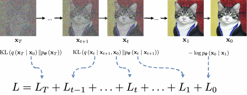
 ; since
  is a fixed distribution that we want to sample from, this means that LT is a constant and can be ignored;
 either, setting them to
  for some constant
  ; they also develop the noise reparametrization mentioned above somewhat further, obtaining a simple closed form for
  ; namely, they assume that the data consists of integers from 0 to 255 scaled linearly to [-1, 1], which is a natural representation for images, and model
![\[p_{\boldsymbol{\theta}}(\mathbf{x}_{0} | \mathbf{x}_1) = \prod_{i=1}^D\int_{\delta_-\left({x}_0,i\right)}^{\delta_+\left({x}_0,i\right)} \mathcal{N}\left({x}\middle|{\mu}_{\boldsymbol{\theta},i}\left(\mathbf{x}_1\right), \sigma_1^2\right)\mathrm{d} x,\]](https://blog.sergeynikolenko.ru/wp-content/ql-cache/quicklatex.com-c92b31f1e22e0e69bfe494d902e9e69b_l3.svg "Rendered by QuickLaTeX.com")
 goes over the pixels (components of
  ),
),  is the independent decoder model, and the integration limits define an interval of length 1/255 on every side of
  , which is a standard trick to make everything smooth and continuous.
 but only on the marginal distributions
 ![\[q_{\sigma}\left(\mathbf{x}_{1:T} | \mathbf{x}_0\right)= q_{\sigma}\left(\mathbf{x}_{T} | \mathbf{x}_0\right)\prod_{t=2}^T q_{\sigma}\left(\mathbf{x}_{t-1} | \mathbf{x}_{t},\mathbf{x}_0\right).\]](https://blog.sergeynikolenko.ru/wp-content/ql-cache/quicklatex.com-482a6dc2586418ffb010e709109ee38c_l3.svg "Rendered by QuickLaTeX.com")
![\[q_{\sigma}\left(\mathbf{x}_{t} | \mathbf{x}_{t-1},\mathbf{x}_0\right)=\frac{q_{\sigma}\left(\mathbf{x}_{t-1} | \mathbf{x}_{t},\mathbf{x}_0\right)q_{\sigma}\left(\mathbf{x}_{t} | \mathbf{x}_0\right)}{q_{\sigma}\left(\mathbf{x}_{t-1} | \mathbf{x}_0\right)}.\]](https://blog.sergeynikolenko.ru/wp-content/ql-cache/quicklatex.com-3be2d15e4762b401aefac0467145311b_l3.svg "Rendered by QuickLaTeX.com")
 that gets us from
  , we are now approximating the random noise
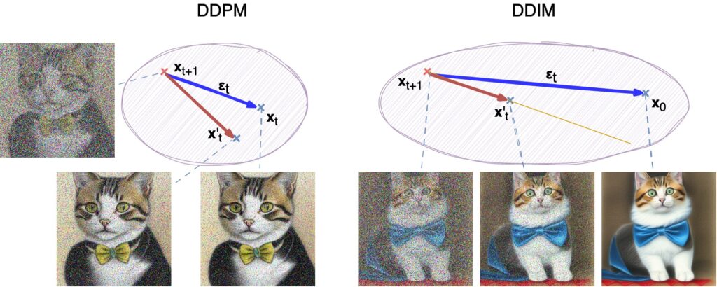
 and the dependence on
  in a single step with correspondingly increased
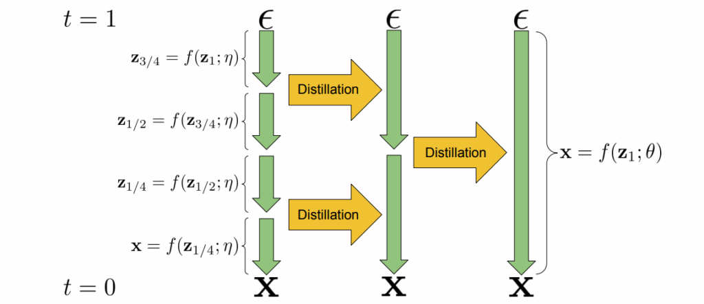
  ! One can train a model with a large number of steps
  but sample only a few of them in the generation part, which speeds things up very significantly. Naturally, the variance will increase, and the approximations will get worse, but with careful tuning this effect can be contained.
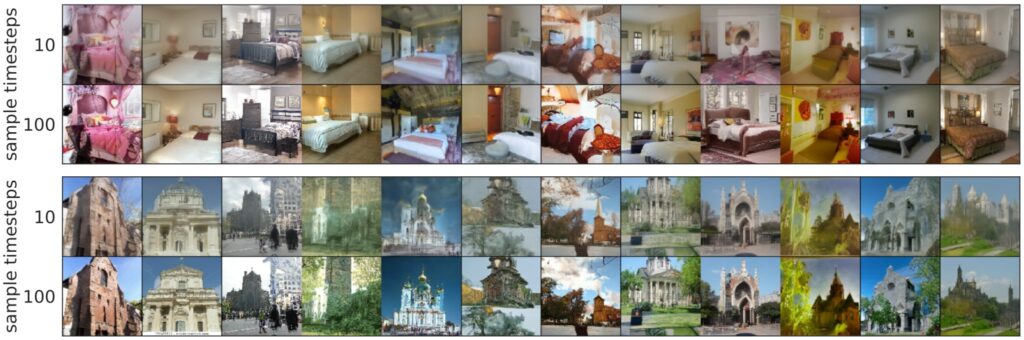
 corresponds to exactly one image, and now we can expect DDIMs to behave in the same way as other models that train latent representations (compare, e.g.,
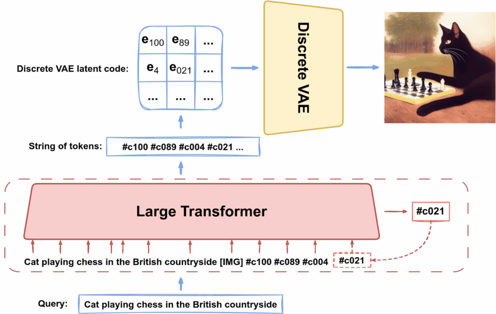
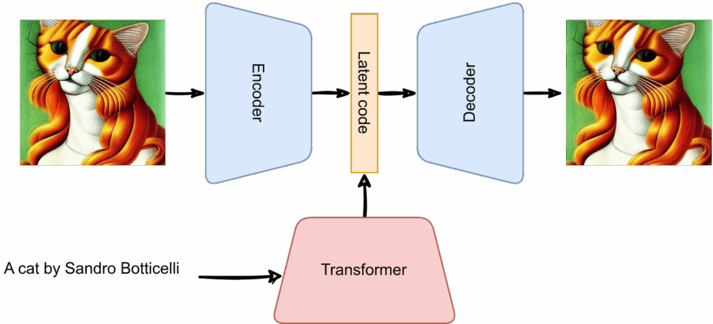
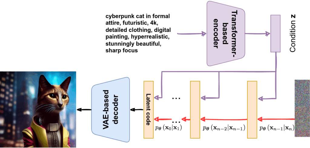
![\[p_{\mathbf{\theta},\mathbf{\psi}}(\mathbf{x},\mathbf{y},\mathbf{z})= p_{\mathbf{\theta}}(\mathbf{x} | \mathbf{y},\mathbf{z})p_{\mathbf{\psi}}(\mathbf{y},\mathbf{z}),\]](https://blog.sergeynikolenko.ru/wp-content/ql-cache/quicklatex.com-665f2cf6c3eb2e073ded3b63cb8692c1_l3.svg "Rendered by QuickLaTeX.com")
 is the corresponding text description, and
  is the image’s latent code. The Transformer learns to generate
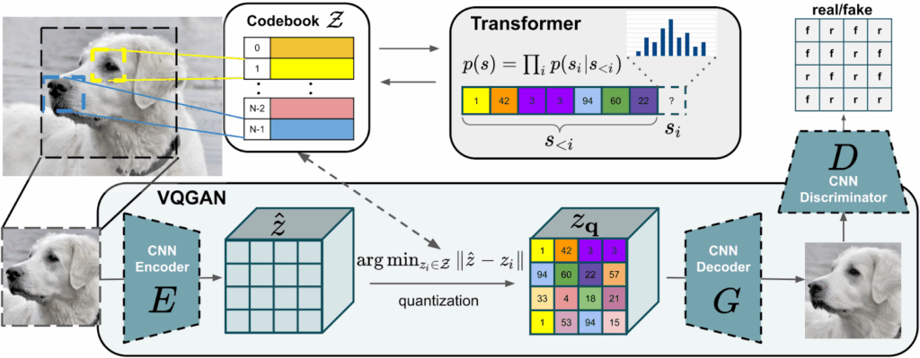
  since it inevitably becomes a generative model for text as well), and the result is used by the discrete VAE, so actually we assume that
  .
.![\[\log p_{\mathbf{\theta},\mathbf{\psi}}(\mathbf{x},\mathbf{y}) \ge \mathbb{E}_{\mathbf{z}\sim q_{\mathbf{\phi}}(\mathbf{z}|\mathbf{x})}\left[ \log p_{\mathbf{\theta}}(\mathbf{x}|\mathbf{y},\mathbf{z}) - \beta\mathrm{KL}\left(q_{\mathbf{\phi}}(\mathbf{z}|\mathbf{x})\| p_{\mathbf{\psi}}(\mathbf{y},\mathbf{z})\right)\right],\]](https://blog.sergeynikolenko.ru/wp-content/ql-cache/quicklatex.com-2c082d6cffd253767b8fe67c9afe5543_l3.svg "Rendered by QuickLaTeX.com")
 is the distribution of latent codes produced by the discrete VAE’s encoder from an image
  here denotes the parameters of the discrete VAE’s encoder;
 is the distribution of images generated by the discrete VAE’s decoder from a latent code
  ;
;  stands for the parameters of the discrete VAE’s decoder;
 is the joint distribution of texts and latent codes modeled by the Transformer; here
  denotes the Transformer’s parameters.
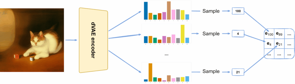
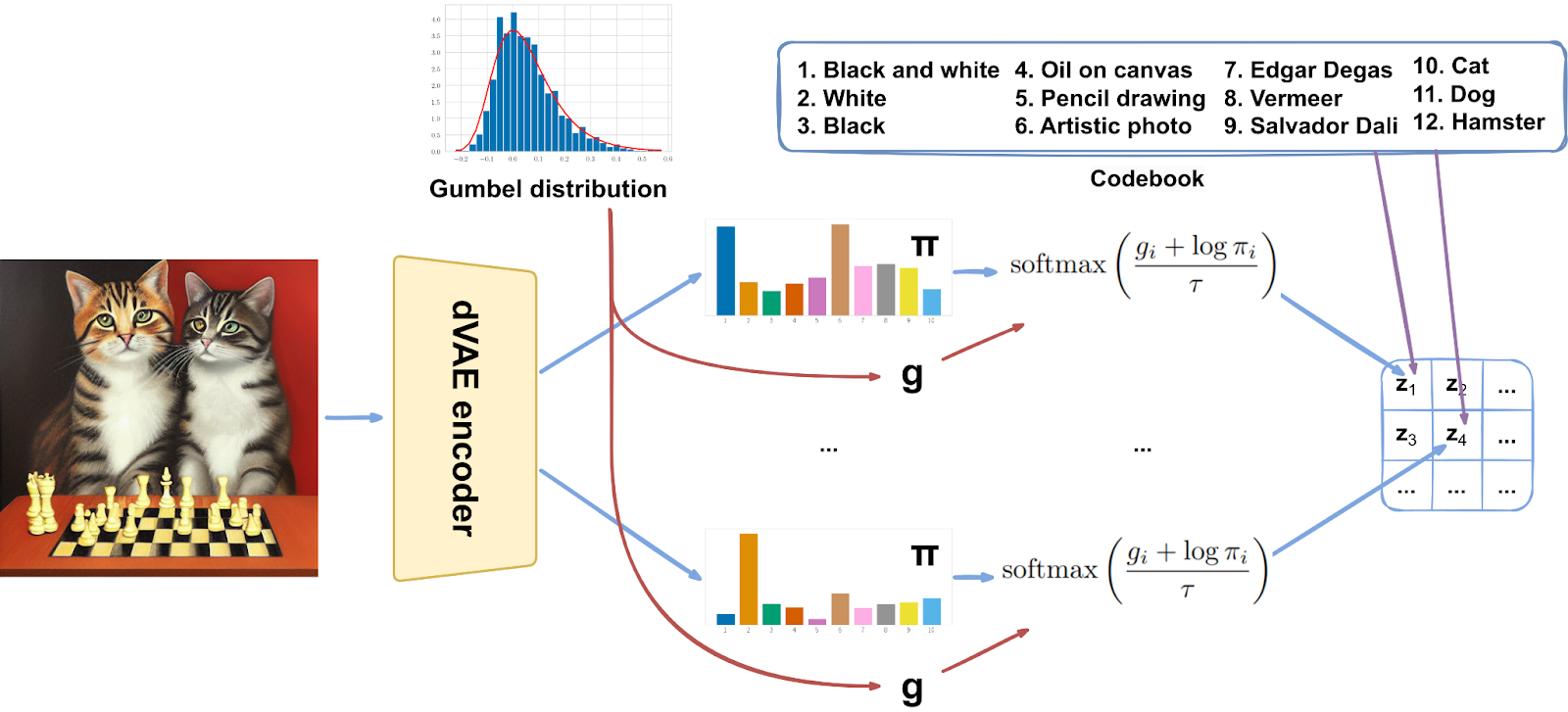
![\[p(g_i) = e^{-\left(g_i + e^{-g_i}\right)},\qquad F(g_i) = e^{-e^{-g_i}}.\]](https://blog.sergeynikolenko.ru/wp-content/ql-cache/quicklatex.com-ba07122ecf12ce18a54348e8eafb06cb_l3.svg "Rendered by QuickLaTeX.com")
![\[z = \arg\,\max_i\left(g_i + \log \pi_i\right).\]](https://blog.sergeynikolenko.ru/wp-content/ql-cache/quicklatex.com-b3f540bcd93d3c6200b013a4585fbfd8_l3.svg "Rendered by QuickLaTeX.com")
![\[y_i = \mathrm{softmax}\left(\frac{1}{\tau}\left(g_i + \log\pi_i\right)\right) = \frac{e^{\frac{1}{\tau}\left(g_i + \log\pi_i\right)}}{\sum_je^{\frac{1}{\tau}\left(g_j + \log\pi_j\right)}}.\]](https://blog.sergeynikolenko.ru/wp-content/ql-cache/quicklatex.com-b62c83de2e58b80c4380e05f88d0c6db_l3.svg "Rendered by QuickLaTeX.com")
 this tends to a discrete distribution with probabilities
  , and during training we can gradually reduce the temperature τ. Note that now the result is not a single codebook vector but a linear combination of codebook vectors with weights
  .
.
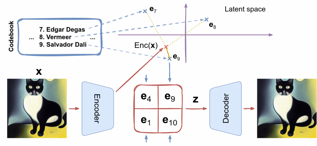
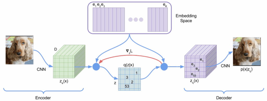
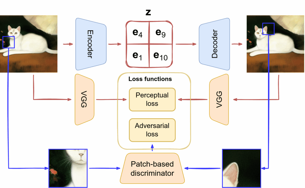
![\[\mathcal{L} = -\log p(\mathbf{x}|\mathbf{z}_q(\mathbf{x}) + \left\|\mathrm{sg}\left[\mathbf{z}_e(\mathbf{x})\right]-\mathbf{e}\right\|_2^2 + \beta\left\|\mathbf{z}_e(\mathbf{x}) - \mathrm{sg}\left[\mathbf{e}\right]\right\|_2^2.\]](https://blog.sergeynikolenko.ru/wp-content/ql-cache/quicklatex.com-00894d566cf8b3d8a7d2f321e7a3f8d8_l3.svg "Rendered by QuickLaTeX.com")
 and
and  are two latent representations for an image
  is the output of the decoder and
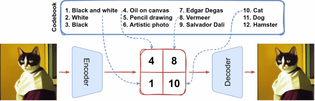
  is the codebook representation after replacing each vector with its nearest codebook neighbor (this notation is illustrated in the image above); the first term is responsible for training the decoder network;
 is the distribution of reconstructed images after the decoder given the latent code; we want the reconstruction to be good so we maximize the likelihood of the original image
  ) and zero during the backward pass (when we compute the gradient
  );
); closer to the latent codes
  can balance the two terms although the authors say that the results don’t change for
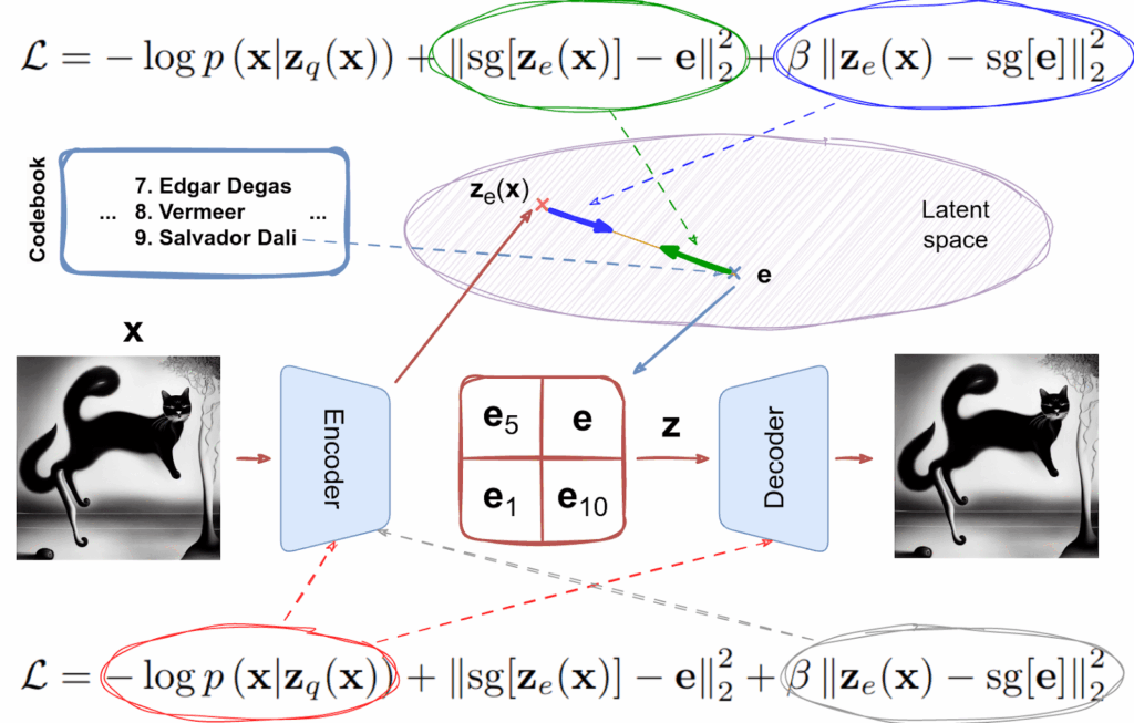


![\[p(\mathbf{z})p(\mathbf{x}|\mathbf{z})=p(\mathbf{x},\mathbf{z})=p(\mathbf{x})p(\mathbf{z}|\mathbf{x})\]](https://blog.sergeynikolenko.ru/wp-content/ql-cache/quicklatex.com-d22a714c241adc27cf598aa1ea0e9c3b_l3.svg "Rendered by QuickLaTeX.com")
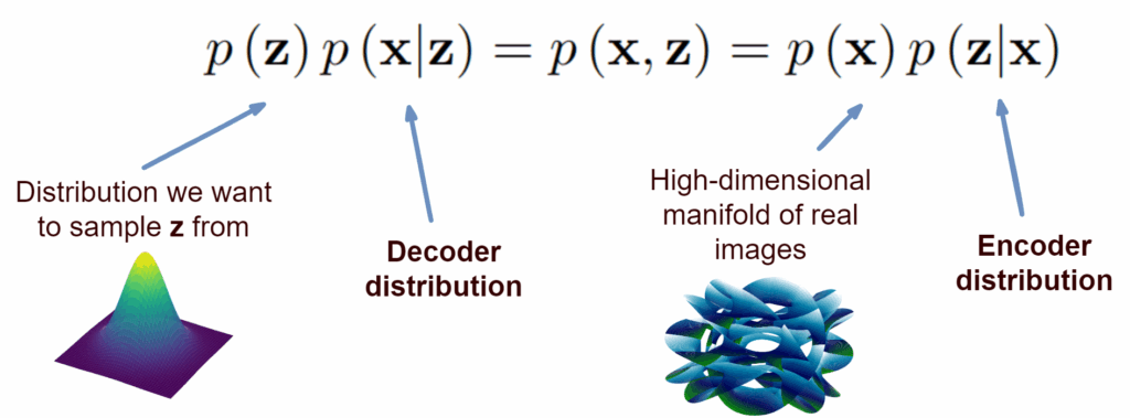
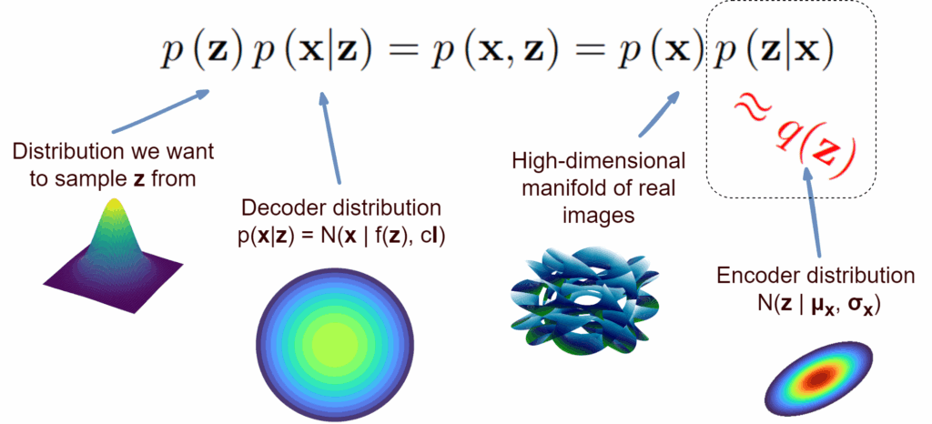
![\[\begin{aligned} p(\mathbf{x},\mathbf{z}) &= p(\mathbf{x})p(\mathbf{z}|\mathbf{x}),\\ \log p(\mathbf{x},\mathbf{z}) &= \log p(\mathbf{x}) + \log p(\mathbf{z}|\mathbf{x}),\\ \log p(\mathbf{x}) &= \log p(\mathbf{x},\mathbf{z}) - \log p(\mathbf{z}|\mathbf{x}),\\\log p(\mathbf{x}) &= \mathbb{E}_{q(\mathbf{z})}\left[\log p(\mathbf{x},\mathbf{z}) - {\log q(\mathbf{z})} + {\log q(\mathbf{z})} - {\log \p(\mathbf{z}|\mathbf{x})\right],\\\log p(\mathbf{x}) &= \int {q(\mathbf{z}}}{\log \frac{p(\mathbf{x},\mathbf{z})}{q(\mathbf{z})}}\dd\mathbf{z} + \int {q(\mathbf{z})}{\log \frac{q(\mathbf{z})}{p(\mathbf{z}|\mathbf{x})}\mathrm{d}\mathbf{z}. \end{aligned}\]](https://blog.sergeynikolenko.ru/wp-content/ql-cache/quicklatex.com-3eace644227b76ee22fff22f10fbbeda_l3.svg "Rendered by QuickLaTeX.com")
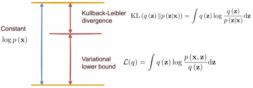
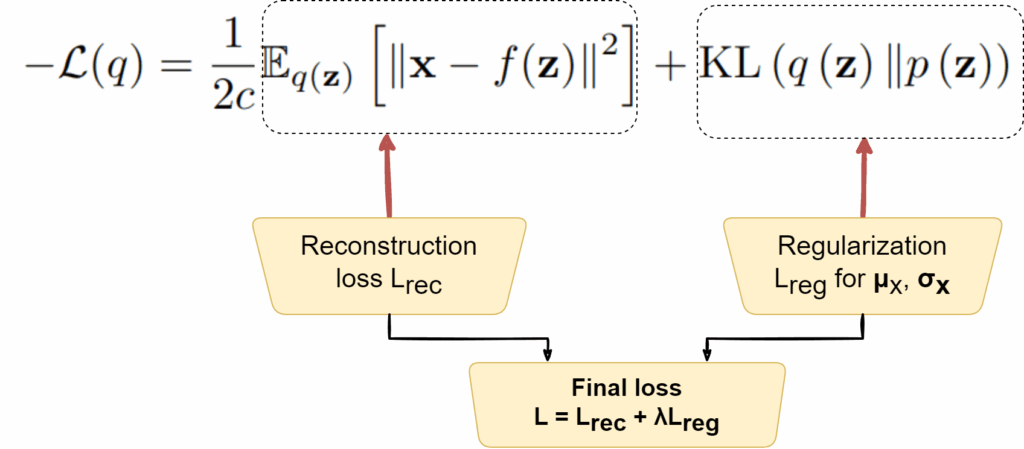
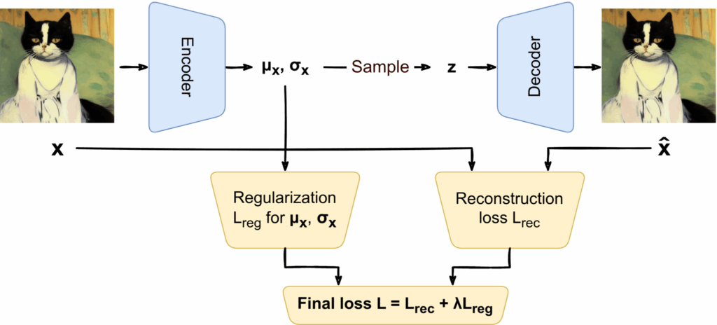
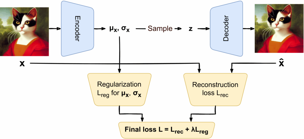
![\[\begin{aligned}\mathcal{L}(q) &= \int {q(\mathbf{z})}{\log \frac{p(\mathbf{x},\mathbf{z})}{q(\mathbf{z})}}\mathrm{d}\mathbf{z} = \int {q(\mathbf{z})}{\log \frac{p(\mathfb{z})p(\mathbf{x}|\mathbf{z})}{q(\mathbf{z})}}\mathrm{d}\mathbf{z} \\&= \int {q(\mathbf{z})}{\log {p(\mathbf{x}|\mathbf{z})}}\mathrm{d}\mathbf{z} + \int {q(\mathbf{z})}{\log \frac{p(\mathbf{z})}{q(\mathbf{z})}}\mathrm{d}\mathbf{z} \\&= \int {q(\mathbf{z})}{\log \mathcal{N}(\mathbf{x}| f(\mathbf{z}),c\mathbf{I})}\mathrm{d}\mathbf{z} - \kl{q(\mathbf{z})}{p(\mathbf{z})} \\&= -\frac{1}{2c}\mathbb{E}_{q(\mathbf{z})}\left[ \left|\mathbf{x} - f(\mathbf{z})\right|^2\right] - \mathrm{KL}\left({q(\mathbf{z})}\|{p(\mathbf{z})}\right).\end{aligned}\]](https://blog.sergeynikolenko.ru/wp-content/ql-cache/quicklatex.com-56f44eeb226e6924c96c9f8bd7fa94a8_l3.svg "Rendered by QuickLaTeX.com")
![\[\mathcal{L} = \mathcal{L}_{\mathrm{rec}} + \lambda\mathcal{L}_{\mathrm{reg}}.\]](https://blog.sergeynikolenko.ru/wp-content/ql-cache/quicklatex.com-767324e9e5f9c0db1d8142be37b299bf_l3.svg "Rendered by QuickLaTeX.com")