We’ve got great news: the very first paper with official Neuromation affiliation has appeared! This work, “3D Molecular Representations Based on the Wave Transform for Convolutional Neural Networks”, has recently appeared in a top biomedical journal, Molecular Pharmaceutics. This paper describes the work done by our friends and partners Insilico Medicine in close collaboration with Neuromation. We are starting to work together with Insilico on this and other exciting projects in the biomedical domain to both significantly accelerate drug discovery and improve the outcomes of clinical trials; by the way, I thank CEO of Insilico Medicine Alex Zhavoronkov and CEO of Insilico Taiwan Artur Kadurin for important additions to this post. Collaborations between top AI companies are becoming more and more common in the healthcare space. But wait — the American Chemical Society’s Molecular Pharmaceutics?! Doesn’t sound like a machine learning journal at all, does it? Read on…

Lead Molecules: Educating the Guess

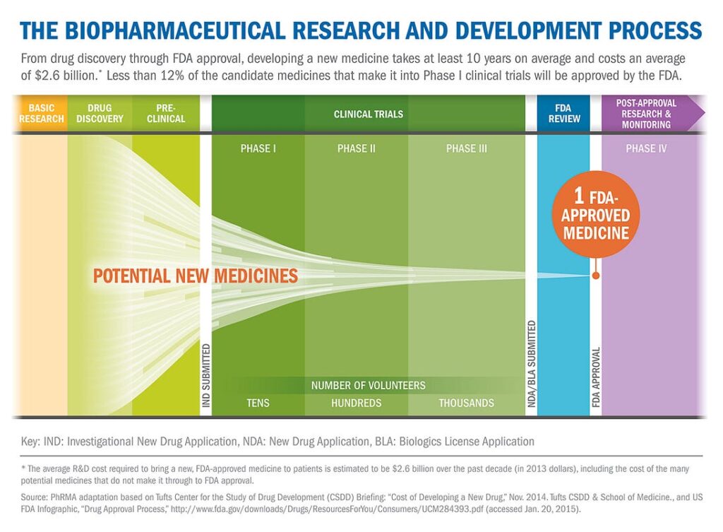
Getting a new drug to the market is a long and tedious process; it can take many years or even decades. There are all sorts of experiments, clinical studies, and clinical trials that you have to go through. And about 90% of all clinical trials in humans fail even after the molecules have been successfully tested in animals.

But to a first approximation, the process is as follows:

• the doctors study medical literature, in particular associations between drugs, diseases, and proteins published in other papers and clinical studies, and find out what the target for the drug should be, i.e., which protein it should bind with;
• after that, they can formulate what kind of properties they want from the drug: how soluble it should be, which specific structures it should have to bind with this protein, should it treat this or that kind of cancer…
• then they sit down and think about which molecules might have these properties; there is a lot to choose from on this stage: e.g., one standard database lists 72 million molecules, complete with their formulas, some properties and everything; unfortunately, it doesn’t always say whether a given molecule cures cancer, this we have to find out for ourselves;
• then their ideas, called lead molecules, or leads, are actually sent to the lab for experimental validation;
• if the lab says that the substance works, the whole clinical trial procedure can be initiated; it is still very long and tedious, and only a small percentage of drugs actually go all the way through the funnel and reach the market, but at least there is hope.

So where is the place of AI in this process? Naturally, we can’t hope to replace the lab or, God forbid, clinical trials: we wouldn’t want to sell a drug unless we are certain that it’s safe and confident that it is effective in a large number of patients. This certainty can only come from actual live experiments. In the future it is likely that we will be able to go from in silico (in a computer) to patients immediately with the AI-driven drug discovery pipelines but today we need to do the experiments.

Note, however, the initial stage of identifying the lead molecules. At this stage, we cannot be sure of anything, but live experiments in the lab are still very slow and expensive, so we would like to find lead molecules as accurately as we can. After all, even if the goal is to treat cancer there is no hope to check the entire endless variation of small molecules in the lab (“small” are molecules that can easily get through a cell membrane, which means basically everything smaller than a nucleic acid). 72 million is just the size of a specific database, the total number of small molecules is estimated to be between 10⁶⁰ and 10²⁰⁰, and synthesizing and testing a single new molecule in the lab may cost thousands or tens of thousands of dollars. Obviously, the early guessing stage is really, really important.

By now you can see how it might be beneficial to apply latest AI techniques to drug discovery. We can use machine learning models to try and choose the molecules that are most likely to have desired properties.

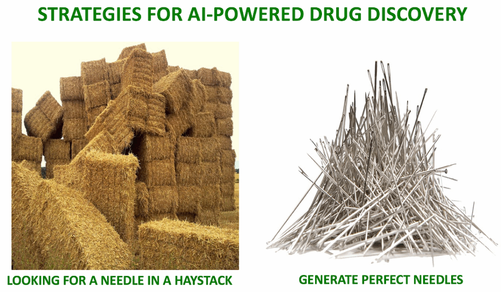
But when you have 72 million of something, “choosing” ceases to look like classification and gets more into the “generation” part of the spectrum. We have to basically generate a molecule from scratch, and not just some molecule, but a promising candidate for a drug. With modern generative models, we can stop searching for a needle in a haystack and design perfect needles instead:

How do we generate something from scratch? Deep learning does have a few answers when it comes to generative models; in this case, the answer turned out to be…

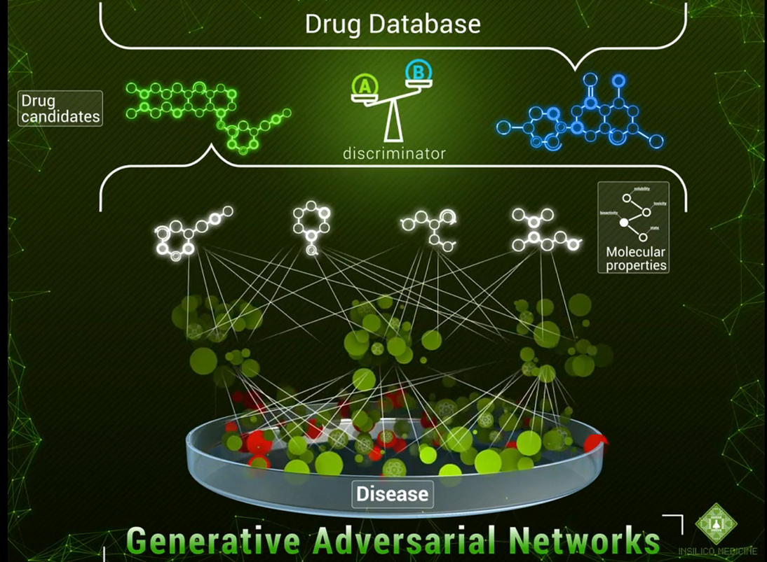
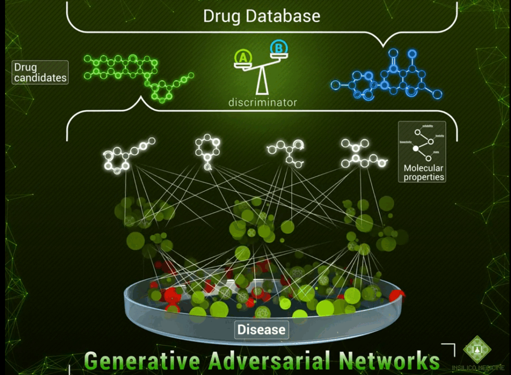
Generative Adversarial Networks

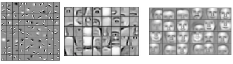
We have already briefly talked about generative adversarial networks (GANs) in a previous post, but I’m sure a reminder is in order here. GANs are a class of neural networks that aim to learn to generate objects from a certain class. Previously, GANs had been mostly used to generate images: human faces as in (Karras et al., 2017), photos of birds and flowers as in StackGAN, or, somewhat suprisingly, bedroom interiors, a very popular choice for GAN papers due to a commonly used part of the standard LSUN scene understanding dataset. Generation in GANs is based on a very interesting and rather commonsense idea. They have two parts that are in competition with each other:

• the objective of the generator is to generate new objects that are supposed to pass for “true” data points;
• while the discriminator has to decipher the tricks played by the generator and distinguish between real data points and the ones produced by the generator.

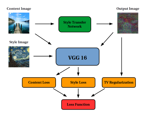
Here is how the general scheme looks:

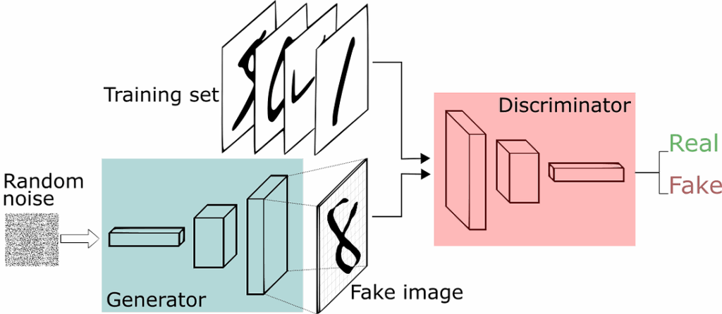
In other words, the discriminator learns to spot the generator’s counterfeit images, while the generator learns to fool the discriminator. I refer to, e.g., this post for a simple and fun introduction to GANs.

We at Neuromation are following GAN research with great interest due to many possible exciting applications. For example, conditional GANs have been used for image transformations with the explicit purpose of enhancing images; see, e.g., image de-raining recently implemented with GANs in this work. This ties in perfectly with our own ideas of using synthetic data for computer vision: with a proper conditional GAN for image enhancement, we might be able to improve synthetic (3D-rendered) images and make them more like real photos, especially in small details. In the post I referred to, we saw how NVIDIA researchers introduced a nice way to learn GANs progressively, from small images to large ones.

But wait. All of this so far makes a lot of sense for images. Maybe it also makes sense for some other relatively “continuous” kinds of data. But molecules? The atomic structure is totally not continuous, and GANs are notoriously hard to train for discrete structures. Still, GANs did prove to work for generating molecules as well. Let’s find out how.

Adversarial Autoencoders

Our recent paper on molecular representations is actually a part of a long line of research done by our good friends and partners, Insilico Medicine. It began with Insilico’s paper “The cornucopia of meaningful leads: Applying deep adversarial autoencoders for new molecule development in oncology”, whose lead author Artur Kadurin is a world-class expert on deep learning, one of Insilico Medicine’s Pharma.AI team on deep learning for molecular biology, recently appointed CEO of Insilico Taiwan… and my Ph.D. student.

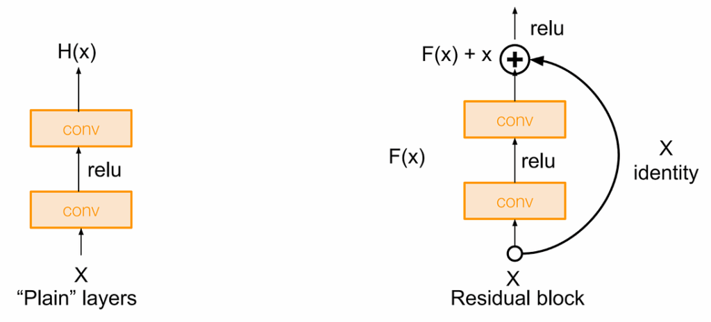
In this work, Kadurin et al. presented an architecture for generating lead molecules based on a variation of the GAN idea called Adversarial Autoencoders (AAE). In AAE, the idea is to learn to generate objects from their latent representations. Generally speaking, autoencoders are neural architectures that take an object as input… and try to return the same object as output. Doesn’t sound too hard, but the idea is that in the middle of the architecture, the input must go through a middle layer that learns a latent representation, i.e., a set of features that succinctly encode the input in such a way that afterwards subsequent layers can decode the object back:

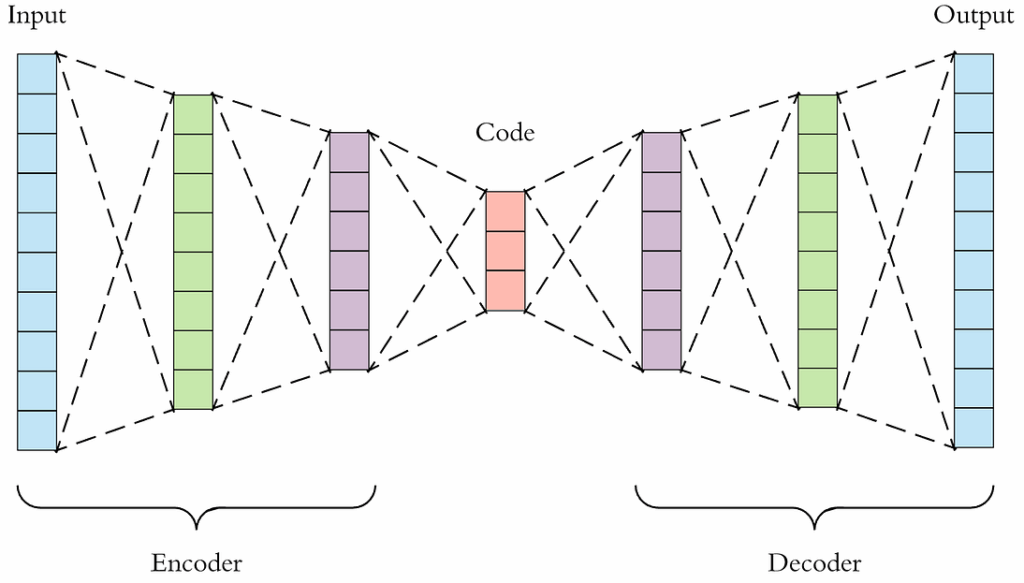
Either the middle layer is simply smaller (has lower dimension) than input and output, or the autoencoder uses special regularization techniques, but in any case it’s impossible to simply copy the input through all layers, and the autoencoder has to extract the really important stuff.

So what did Kadurin et al. do? They took a conditional adversarial autoencoder and trained it to generate fingerprints of molecules, using and serving desired properties as conditions. Here is the general model architecture from (Kadurin et al., 2017):

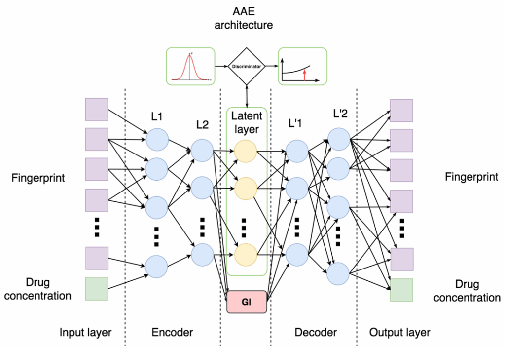
Looks just like the autoencoder above, but with two important additions in the middle:

• on top, there is a discriminator that tries to distinguish the distribution of latent representations from some standard distribution, e.g., a Gaussian; this is the main idea of AAE: if you can make the distribution of latent codes indistinguishable from some standard distribution, it means that you can then sample from this distribution and generate reasonable samples through the decoder;
• on the bottom, there is a condition that in this case encodes desired properties of the molecule; we train on the molecules with known properties, and the problem is then to generate molecules with desired (perhaps even never before seen) combinations of properties.

There is still that nagging question about the representations, though. How do we generate discrete structures like molecules? We will discuss molecular representations in much greater detail in the next post; here let me simply mention that this work used a standard representation of a molecule as a MACCS fingerprint, a set of binary characteristics of the molecule such as “how many oxygens is has” or “does it have a ring of size 4”.

Basically, the problem becomes to “translate” the condition, i.e., desired properties of a molecule, into more “low-level” properties of the molecular structure encoded into their MACCS fingerprints. Then a simple screening of the database can find molecules with the fingerprints most similar to generated ones.

At the time that was the first peer-reviewed paper showing that GANs can generate novel molecules. The submission was made in June 2016 and it was accepted in December 2016. In 2017 the community started to notice:

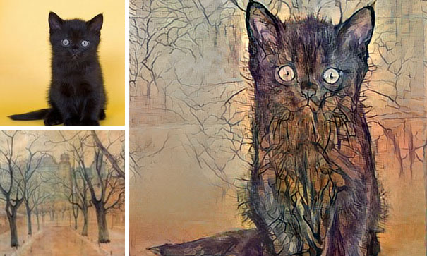
It turned out that the resulting molecules do look interesting…

Conclusion

This post is getting a bit long; let’s take it one step at a time. We will get to our recent paper in the next installment, and now let us summarize what we’ve seen so far.

Since the deep learning revolution, deep neural networks have been revolutionizing one field after another. In this post, we have seen how modern deep learning techniques are transforming molecular biology and drug discovery. Constructions such as adversarial autoencoders are designed to generate high-quality objects of various nature, and it’s not a huge wonder that such approaches work for molecular biology as well. I have no doubt that in the future, these or similar techniques will bring us closer to truly personalized medicine.

So what next? Insilico has already generated several very promising candidates for really useful drugs. Right now they are undergoing experimental validation in the lab. Who know, perhaps in the next few years we will see new drugs identified by deep learning models. Fingers crossed.

Sergey Nikolenko
Chief Research Officer, Neuromation

In the fourth installment of the NeuroNuggets series, we continue our study of basic problems in computer vision. We remind that in the NeuroNuggets series, we discuss the demos available on the recently released NeuroPlatform, concentrating not so much on the demos themselves but rather on the ideas behind each deep learning model.

In the first installment, we talked about the age and gender detection model, which is basically image classification. In the second, we presented object detection, a more complex computer vision problem where you also have to find where an object is located. In the third, we continued this with segmentation and Mask R-CNN model. Today, we turn to something even more exciting. We will consider a popular and very beautiful application of deep learning: style transfer. We will see how to make a model that can draw your portrait in the style of Monet — or Yves Klein if you’re not careful with training! I am also very happy to present the co-author of this post, one of our lead researchers Kyryl Truskovskyi:

Style Transfer: the Problem

Imagine that you can create a true artwork by yourself, turning your own photo or a familiar landscape into a painting done like Van Gogh or Picasso would do it. Sounds like a pipe dream? With the help of deep neural networks, this dream has now become reality. Neural style transfer has become a trending topic both in academic literature and industrial applications; we all know and use popular mobile apps for style transfer and image enhancement. Starting from 2014, these style transfer apps have become a huge PR point for deep neural networks, and today almost all smartphone users have tried some style transfer app for photos and/or video. By now, all of these methods work in real-time and run on mobile devices, and anyone can create artwork with a simple app, stylizing their own images and videos… but how do these apps work their magic?

From the deep learning perspective, ideas for style transfer stem from attempts to interpret the features that a deep neural network learns and understand how exactly it works. Recall that a convolutional neural network for image processing gradually learns more and more convoluted features (see, e.g., our first post in the NeuroNuggets series), starting from basic local filters and getting all the way to semantic features like “dog” or “house”… or, quite possibly, “Monet style”! The basic idea of style transfer is to try to disentangle these features, pull apart semantic features of “what is on the picture” from “how the picture looks”. Once you do it, you can try to replace the style while leaving the contents in place, and the style can come from a completely different painting.

For the reader interested in a more detailed view, we recommend “Neural Style Transfer: A Review”, a detailed survey of neural style transfer methods. E.g., here is an example from that paper where a photo of the Great Wall of China has been redone in classical Chinese painting style:

And here is an example from DeepArt, one of the first style transfer services:

You can even do it with videos:

But let’s see how it works!

Neural Style Transfer by Optimizing the Image

There are two main approaches to neural style transfer: optimization and feedforward network. Let us begin with optimization.

In this approach, we optimize not the network but the resulting image. This is a very simple but powerful idea: the image itself is also just a matrix (tensor) of numbers, just like the weights of the network. This means that we can take derivatives with respect to these weights, extending backpropagation to them too and optimizing an image for a network rather then the other way around; we have already discussed this idea in “Can a Neural Network Read Your Mind?”.

For style transfer, it works as follows: you have a content image, style image and trained neural network (on ImageNet for example). You create a newly generated image, initializing it completely at random. Then the content image and style image pass through the early and intermediate layers of the network to compute two types of loss functions: style loss and content loss (see below). Next, we optimize their losses by changing the generated image, and after a few iterations we have beautiful stylized images. The structure is a bit intimidating:

But do not worry — let’s talk about the losses. After we pass an image through a network we get a feature map from intermediate layers. This feature map captures the semantic representation of this image. And we definitely want the new image to be similar to the content image, so for content image feature maps C and generated image feature maps P we get the following content loss:

The style loss is slightly different: for the style loss we compute Gram matrices of the intermediate representations of generated images and style image:

The style loss is the Euclidean distance between Gram matrices

By directly minimizing the sum of these losses by gradient descent on our generated image, we make it more and more similar to the style image in terms of style while still keeping the content due to the content loss. We refer to the original paper, “A Neural Algorithm of Artistic Style”, for details. This approach works great, but its main disadvantage is that it takes a lot of computational effort.

Neural Style Transfer Via Image Transformation Networks

The basic idea for the next is to use feed-forward networks for image transformation tasks. Basically, we want to create an image transformation network that would directly create beautiful stylized images, with no complicated “image training” process.

The algorithm is simple. Suppose that, again, you have a content image and a style image. You feed the content image through the image transformation network and get a new generated image. After that, loss networks are used to compute style and content losses, like in the optimization method above, but after that, we optimize not the image itself but the image transformation network. This way, we get a trained image transformation network for style transfer and then can use it for stylizing as only a forward pass without any optimization at all.

Here is how it looks through the entire process with the image transformation network and the loss network:

The original paper on this approach, “Perceptual Losses for Real-Time Style Transfer and Super-Resolution”, led to the first truly popular and the first real-time implementation of style transfer and superresolution algorithms; you can find a sample code for this approach here. The image transformation network works fast, but its main disadvantage is that we need to train a completely separate new network for every style image. This is not a problem for preset instagram-like filters but does not solve the general problem.

To fix this, authors of “A Learned Representation for Artistic Style” introduced an approach called conditional instance normalization. The basic idea is to train one network for several different styles. It turns out that normalization plays a huge role in style networks to model a style, and it is sufficient to specialize scaling and shifting parameters after normalization to each specific style. In simpler words, it is enough just to tune the parameters of a simple transformation after normalization for each style, before image transformation network.

Here is a picture of how it works; for the mathematical details, we refer to the original paper:

You can find an example code for this model here.

In the platform demo, we use the Python framework PyTorch for training the neural networks, Flask + Gunicorne to serve it on our platform, and Docker + Mesos for deploying and scaling.

Try it out on the platform

Now that we know about style transfer, it is even better to see the result for ourselves. We follow the usual steps to get the model working.

1. Login at https://mvp.neuromation.io
2. Go to “AI Models”:

3. Click “Add more” and “Buy on market”:

4. Select and buy the Image Style Transfer demo model:

5. Launch it with the “New Task” button:

6. Try the demo! You can upload your own photo for style transfer. We chose this image:

Neuromation Team in Singapore

7. And here you go!

Stylized and enhanced Neuromation Team in Singapore

And here we are:

Sergey Nikolenko
Chief Research Officer, Neuromation

Kyryl Truskovskyi
Lead Researcher, Neuromation

In the third post of the NeuroNuggets series, we continue our study of basic problems in computer vision. I remind the reader that in this series we discuss the demos available on the recently released NeuroPlatform, concentrating not so much on the demos themselves but rather on the ideas behind each deep learning model. This series is also a great chance to meet the new Neuromation deep learning team that has started working at our new office in St. Petersburg, Russia.

In the first installment, we talked about the age and gender detection model, which is basically image classification. In the second, we presented object detection, a more complex computer vision problem where you also have to find where an object is located. Today, we continue with segmentation, the most detailed problem of this kind, and consider the latest addition to the family of R-CNN models, Mask R-CNN. I am also very happy to present the co-author of this post, Anastasia Gaydashenko:

Segmentation: Problem Setting

Segmentation is a logical next step of the object detection problem that we talked about in our previous post. It still stems from the same classical computer vision conundrum: even with great feature extraction, simple classification is not enough for computer vision, you also have to understand where to extract these features. Given a photo of your friends, a landscape scene, or basically any other image, can you automatically locate and separate all the objects in the picture? In object detection, we looked for bounding boxes, i.e., rectangles that enclose the objects. But what if we require more detail and label the exact silhouettes of the objects, excluding background? This problem is called segmentation. Generally speaking, we want to go from pictures in the first row to pictures in the second row on this picture:

Formally speaking, we want to label each pixel of an image with a certain class (tree, road, sky, etc) as shown in the image. The first question, of course, is why? What’s wrong with regular object detection? Actually, segmentation is applied widely: in medical imaging, сontent-based image retrieval, and so on. It avoids the big problem of regular object detection: overlapping bounding boxes for different objects. If you see three heavily overlapping bounding boxes, are these three different hypotheses for the same object (in which case you should choose one) or three different objects that happen to occupy the same rectangle (in which case you should keep all three)? Regular object detection models can’t really decide.

And if the shape of the object is far from rectangular segmentation provides much better information (this is very important for medical imaging). For instance, Google used semantic image segmentation to create the Portrait Mode in its signature Pixel 2 phone.

These pictures also illustrate another important point: the different flavours of segmentation. What you see above is called semantic segmentation; it’s the simpler version, when we simply want to classify all pixels to categories such as “person”, “airplane”, or “background”. You can see in the picture above that all people are labeled as “person”, and the silhouettes blend together into a big “cuddle pile”, to borrow the expression used in certain circles.

This leads to another, more detailed type of segmentation: instance segmentation. In this case, we would want to separate the people in the previous photo and label them as “person 1”, “person 2”, etc., as shown below:

Here all people on the photo are marked in different colors, which mean different instances. Note also that they are labeled with probabilities that reflect the model’s confidence in a particular class label; the confidence is very high in this case, but generally speaking it is also a desirable property of any AI model to know when it is not sure.

Convolutions and Convolutional Neural Networks

So how can a computer vision system parse these images in such an accurate and humanlike way? Let’s find out. The first thing we need to study is how convolution works and why do we use it. And yes, we return to CNNs in each and every post — because they are really important and we keep finding new things to say about them. But before we get to the new things, let’s briefly go through the old, concentrating on the convolutions themselves this time.

Initially, the idea of convolution has come from biology, or, more specifically, studies of the visual cortex. David Hubel and Torsten Wiesel studied the lower layers of the visual cortex in cats. Cat lovers, please don’t watch this:

https://cdn.embedly.com/widgets/media.html?src=https%3A%2F%2Fwww.youtube.com%2Fembed%2FYoo4GWiAx94%3Ffeature%3Doembed&url=http%3A%2F%2Fwww.youtube.com%2Fwatch%3Fv%3DYoo4GWiAx94&image=https%3A%2F%2Fi.ytimg.com%2Fvi%2FYoo4GWiAx94%2Fhqdefault.jpg&key=a19fcc184b9711e1b4764040d3dc5c07&type=text%2Fhtml&schema=youtube

When Hubel and Wiesel moved a bright line across a cat’s retina, they noticed an interesting effect: the activity of neurons in the brain changed depending on the orientation of the line, and some of the neurons fired only when the line was moving in a particular direction. In simple terms, that means that different regions of the brain react to different simple shapes. To model this behaviour, researchers had to invent detectors for simple shapes, elementary components of an image. That’s how convolutions appeared.

Formally speaking, convolution is just a scalar product of two matrices taken as vectors: we multiply them componentwise and sum up the results. The first matrix is called the “kernel”; it represents a simple shape, like this one:

The second matrix is just some patch from the picture where we want to find the pattern shown in the kernel. If the convolution result is large, we decide that the target shape is indeed present in this patch. Then we can simply run the convolution through all patches in the image and detect where the pattern occurs.

For example, let us try to find the filter above in a picture of a mouse. Here you can see the part where we would expect the filter to light up:

And if we multiply the corresponding submatrix with the kernel and sum all the values, we indeed get a pretty big number:

On the other hand, a random part of the picture does not produce anything at all, which means that it is totally different from the filter’s pattern:

Filters like this let us detect some simple shapes and patterns. But how do we know which of these forms we want to detect? And how can we recognize a plane or an umbrella from these simple lines and curves?

This is exactly where the training of the neural networks comes in. The shapes defined by kernels (the filters) are actually what the CNN learns from the training set. It is usually simple lines and gradients on the first layers of the neural network, but then, with each layer of the model, these shapes are combined with one another into recognizable kernels; a set of kernels is called a map:

The other operation necessary for CNNs is pooling. It is mostly used to reduce computational costs and suppress noise. The main idea is to cover a matrix with small submatrices and leave only one number in each, thus reducing the dimension; usually, the result is just a maximum or average of the values in the small submatrix. Here is a simple example:

This kind of operations is also sometimes called downsampling as they reduce the amount of information we store.

The R-CNN models and Mask R-CNN

Above, we have seen a simplified explanation of techniques used to create convolutional neural networks. We have not touched upon learning at all, but that part is pretty standard. With these simple tools, we can teach a computer model to recognize all sorts of shapes; moreover, CNNs operate on small patches so they are perfectly parallelizable and well suited for GPUs. We recommend our previous two posts for more details on CNNs, but let us now move on to the more high-level things, that is, segmentation.

In this post, we do not discuss all modern segmentation models (there are quite a few) but go straight to the model used in the segmentation demo on the NeuroPlatform. This model is called Mask R-CNN, and it is based on the general architecture of R-CNN models that we discussed in the previous post about object detection; hence, a brief reminder is again in order.

It all begins with the R-CNN model, where R stands for “region-based”. The pipeline is pretty simple: we take a picture and apply an external algorithm (called selective search) to it, searching for all kind of objects. Selective search is a heuristic method that extracts regions based on connectivity, color gradients, and coherence of pixels. Next, we classify all extracted regions with some neural network:

Due to the high number of proposals, R-CNN worked extremely slow. In Fast R-CNN, the RoI (region of interest) projection layer was added to the neural network: instead of putting each region from proposals through the whole network, Fast R-CNN takes the whole image through the network once, finds neurons corresponding to a particular region in the feature map in the network, and then applies the remaining part of the network to each found set of neurons. Like here:

The next step was to invent the Region Proposal Network that could replace selective search; the Faster R-CNN model is now a complete end-to-end neural network.

You can read about all these steps in more detail in our object detection post. But we’re here to learn how Faster R-CNN can be converted to solve the segmentation problem! Actually, it is extremely simple but nevertheless efficient and functional. The authors just added a parallel branch for predicting an object mask to the original Faster R-CNN model. Here is how the resulting Mask R-CNN model looks like:

The top branch in the picture predicts the class of some region and the bottom branch tries to label each pixel of the region to construct a binary mask (i.e., object vs. background). It only remains to understand where this binary mask comes from.

Fully Convolutional Networks

Let us take a closer look at the segmentation part. It is based on a popular architecture called Fully Convolutional Network (FCN):

The FCN model can be used for both image detection and segmentation. The idea is pretty straightforward, and the network is actually even simpler than usual, but it’s still a deep and interesting idea.

In standard deep CNNs for image classification, the last layer is usually a vector of the same size as the number of classes that shows the “scores” of different classes that could be then normalized to give class probabilities. This is what happens in the “class box” on the picture above.

But that if we stop at some middle layer of the CNN and instead of vectors do some more convolutions? And on the last convolutional layer, we get the same number of features as the number of classes. Then, after proper training, we can get “class scores” in every pixel of the last layer, getting a kind of a “heatmap” for every class! Here is how it works — regular classification on top and a fully convolutional approach on the bottom:

For segmentation via this network, we will use the inverses of convolution and pooling. Meet… deconvolution and unpooling!

In deconvolution, we basically do convolution but the matrix is transposed, and now the output is a window rather than a number. Here are two popular ways to do deconvolution (white squares are zero paddings), animated for your viewing convenience:

To understand unpooling, recall the pooling concept that we discussed above. To do max-pooling, we take the maximum value from some submatrix. Now we want to also remember the coordinates of the cells from which we took it and then use it to “invert” max-pooling. We create the matrix with the same shape as the initial and put maximums to the corresponding cells, reconstructing other cell values with approximations based on known cells. Some information stays lost, of course, but usually upsampling works pretty well:

Through the use of deconvolution and unpooling, we can construct pixel-wise predictions for each class, that is, segmentation masks for the image!

Segmentation demo in action

We have seen how Mask R-CNN does segmentation, but it is even better to see the result for yourself. We follow the usual steps to get the model working.

1. Login at https://mvp.neuromation.io
2. Go to “AI Models”:

3. Click “Add more” and “Buy on market”:

4. Select and buy the Object Segmentation demo model:

5. Launch it with the “New Task” button:

6. Try the demo! You can upload your own photo for segmentation. We chose this image:

7. And here you go! The model shows bounding boxes as well, but now it gives much more than just bounding boxes:

Sergey Nikolenko
Chief Research Officer, Neuromation

Anastasia Gaydashenko
Junior Researcher, Neuromation

Neuromation’s global team gathered in Tel-Aviv at the Future of AI conference to present our concept of Knowledge Mining to the international AI market. Israel has taken a promising position in AI, creating nearly 700 AI jobs, of which only 300 were filled.

This is an example of the growing demand for AI talent and products that Neuromation is filling through its distributed marketplace Platform, and its custom turn-key solutions provided by Neuromation Labs.

Stay with us, more reports from the event, including the recording of the keynote speech by Maxim Prasolov, CEO and Sergey Nikolenko, CRO, are coming soon.

This is the second post in our NeuroNuggets series. This is a series were we discuss the demos already available on the recently released NeuroPlatform. But it’s not as much about the demos themselves as about the ideas behind each of these models. We also meet the new Neuromation deep learning team that we hired at our new office in St. Petersburg, Russia.

The first installment was devoted to the age and gender estimation model, the simplest neural architecture among our demos, but even there we had quite a few ideas to discuss. Today we take convolutional neural networks for image processing one step further: from straightforward image classification to object detection. It is also my pleasure to introduce Aleksey Artamonov, one of our first hires in St. Petersburg, with whom we have co-authored this post:

Object Detection: Not Quite Trivial

Looking at a picture, you can recognize not only what objects are on it, but also where they are located. On the other hand, a simple convolutional neural network (CNN) like the one we considered in the previous post cannot do that. All they can is estimate the probability with which a given object is present on the image. For practical purposes, this is insufficient: on real world images, there are lots of objects that can interact with each other in nontrivial ways. We need to ascertain the position and class of each object in order to extract more semantic information from the scene. We have already seen it with face detection:

The simplest approach that was used before the advent of convolutional networks consisted of a sliding window and a classifier. If we need, say, to find human faces on a photo, we first train a network that says how likely it is that a given picture contains a face and then apply it to every possible bounding box (a rectangle in the photo where an object could appear), choosing the bounding boxes where this probability is highest.

This approach actually would work pretty well… if anyone could apply it. Detection with a sliding window needs to look through a huge amount of different bounding boxes. Bounding boxes have different positions, aspect ratios, scales. If we try to calculate all the options that we should look through, we get about 10 million combinations for a 1Mpix image. Which means that the naive approach would need to run the classification network 10 million times to detect the actual position of the face. Naturally, this would never do.

Classical Computer Vision: the Viola-Jones Algorithm

Our next stop is an algorithm that embodies classical computer vision approaches to object detection. By “classical” here we mean computer vision as it was before the deep learning revolution made every kind of image processing into different flavours of CNNs. In 2001 Paul Viola and Michael Jones proposed an algorithm for real-time face detection. It employs three basic ideas:

• Haar feature selection;
• boosting algorithm;
• cascade classifier.

Before describing these stages, let us make sure that we actually want the algorithm to achieve. A good object detection algorithm has to be fast and have a very low false-positive rate. We have 10 million possible bounding boxes and only a handful of faces on the photo, so we cannot afford a false positive rate much higher than 10–6 unless we want to be overwhelmed by incorrect bounding boxes. With this in mind, let us jump into the algorithm.

The first part is the Haar transform; it is best to begin with a picture:

We overlap different filters on our image. Activation of one Haar filter is the sum of the values in the white parts of the rectangle minus the sum of values under black part.

The main property of these filters is that they can be computed across the entire image very quickly. Let us consider the integral version (I*) of the original image (I); the integral version is the image where intensity at coordinate I*x,y is the total intensity over the whole rectangle that begins at the top left corner and ends in (x,y):

Let us see the Haar filter overlapped on the image and its integral version in action:

Haar features for this filter could be computed in just a few operations. E.g., the horizontal Haar filter activation shown on the Terminator’s face equals 2C — 2D + B — A + F — E, where the letters denote intensities at the corresponding points on the integral image. We won’t go into the formulas but you can check it yourself, it’s a good exercise for understanding the transform.

To select the best Haar features for face recognition, the Viola-Jones algorithm uses the AdaBoost classification algorithm. Boosting models (in particular, AdaBoost) are machine learning models that combine and build upon simpler classifiers. AdaBoost can take weak features like Haar that are just a little better than tossing a coin. But then AdaBoost learns a combination of these features in such a way that the final decision rule is much stronger and better. It would take a whole separate post to explain AdaBoost (perhaps we should, one day), so we’ll just add a couple of links and leave it at that.

The third, final idea is to combine the classifiers into a cascade. Thing is, even boosted classifiers still have too much false positives. A simple 2-feature classifier can achieve almost 100% detection rate, but with a 50% false positive rate. Therefore, the Viola-Jones algorithm uses a cascade of gradually more complex classifiers, where we can reject a bounding box on every step but have to pass all checks to output a positive answer:

This approach leads to much better detection rates. Roughly speaking, if we have 10 stages in our cascade, each stage has 0.3 false positive rate and 0.01 false negative rate, and all stages are independent (this is a big assumption, of course, but in practice it still works pretty well), the resulting cascade classifier achieves (0.3)¹⁰ ~ 3*10^–6 false positive rate and 0.9 detection level. Here is how a cascade works on a group photo:

Further research in classical computer vision went into detecting objects of specific classes such as pedestrians, vehicles, traffic signs, faces etc. For complex detectors on deep phases of a cascade we can use different kinds of classifiers such as histogram of oriented gradients (HOG) or support vector machines (SVM). Instead of using Haar features on image in grayscale we can get image channels in different color schemes (CIELab or HSV) and image gradients in different directions. All these features are computed in the integral space, summing inside a rectangle with an adjustable threshold.

An important problem that appeared already in classical computer vision is that near a real object, our algorithms will find multiple intersecting bounding boxes; you can draw different rectangles around a given face, and all will have rather high confidence. To choose the best one classical computer vision usually employs the non-maximum suppression algorithm. However, this still remains an open and difficult problem because there are many situations when two or more objects have intersecting bounding boxes, and a simple greedy implementation of non-maximum suppression would lose good bounding boxes. This part of the problem is relevant for all object detection algorithms and still remains an active area of research.

R-CNN

Initially, in object detection tasks neural networks were treated as tools for extracting features (descriptors) on late stages of the cascade. Neural networks by themselves had always been very good in image classification, i.e., prediction of the class or type of the object. But for a long time, there was no mechanism to locate this object at the image with neural networks.

With the deep learning revolution, it all changed rather quickly. By now, there are several competing approaches to object detection that are all based on deep neural networks: YOLO (“You Only Look Once”, a model that was initially optimized for speed but ), SSD (single-shot detectors), and so on. We may return to them in later installments, but in this post we concentrate on a single class of object detection approaches, the R-CNN (Region-Based CNN) line of models.

The original R-CNN model, proposed in 2013, performs a three-step algorithm to do object detection:

• generate hypotheses for reasonable bounding boxes with an external region proposal algorithm;
• warp each proposed region in the image and pass it through a CNN trained for image classification to extract features;
• pass the resulting features to a separate SVM classification model that actually classifies the regions and chooses which of them contain meaningful objects.

Here is an illustration from the R-CNN paper:

R-CNN brought the deep learning revolution to object detection. With R-CNN, mean average precision on the Pascal VOC (2010) dataset grew from 40% (the previous record) up to 53%, a huge improvement.

But improved object detection quality is only part of the problem. R-CNN worked well but was hopelessly slow. The main problem was that you had to run the CNN separately for every bounding box; as a result, object detection with R-CNN took more than forty seconds on a modern GPU for a single image! Not quite real-time. It is also very hard to train because you had to juggle together the three components, two of which (CNN and SVM) are machine learning models that you have to train separately. And, among other things, R-CNN requires an external algorithm that can propose bounding boxes for further classification. In short, something had to be done.

Fast R-CNN

The main problem of R-CNN was speed, so when researchers from Microsoft Research rolled out an improvement there was no doubt how to name the new model: Fast R-CNN was indeed much, much faster. The basic idea (we will see this common theme again below) was to put as much as they could directly into the neural network. In Fast R-CNN, the neural network is used for classification and bounding box regression instead of SVM:

In order to make detection independent of the size of the object in the image, R-CNN uses Spatial Pyramid Pooling (SPP) layers that had been introduced in SPPnet. The Idea of SPP is brilliant: instead of cropping and warping the region to construct an input image for a separate run of the classification CNN, SPP crops the region of interest (RoI) projection at deeper convolutional layer, before fully-connected layers.

This means that we can reuse lower layers of the CNN, running it only once instead of a thousand times in basic R-CNN. But a problem arises: a fully-connected layer has a certain size, and the size of our RoI can be anything. The task of the spatial pyramid pooling layer is to solve this problem. The layer divides the window into 21 parts, as shown in the figure below, and summarizes (pools) the values in each part. Thus, the size of the layer’s output does not depend on the size of the input window any more:

Fast R-CNN is 200 times faster than R-CNN to apply to a test image. But it is still insufficient for actual real-time object detection due to an external algorithm for generating bounding box hypotheses. On a real photo, this algorithm can take about 2 seconds, so regardless of how fast we make the neural network, we have at least a 2 second overhead for every image. Can we get out of this bottleneck?

Faster R-CNN

What could be faster than Fast R-CNN? The aptly named Faster R-CNN, of course! And what kind of improvement could we do to Fast R-CNN to get an even faster model? It turns out that we can get rid of the only external algorithm left in the model: extracting region proposals.

The beauty of Faster R-CNN is that we can use the same neural network to extract region proposals. We only need to augment it with a few new layers, called the Region Proposal Network (RPN):

The idea is that the first (nearest to input) layers of a CNN extract universal features that could be useful for everything, including region proposals. On the other hand, the first layers have not yet lost all the spatial information: these features are still rather “local” and correspond to relatively small patches of the image. Thus, RPN uses precomputed feature values from early layers to propose regions with objects for further classification. RPN is a fully convolutional network, and there are no fully-connected layers in the RPN architecture, so the computing overhead is almost nonexistent (10ms per image), and we can now completely remove the region proposal algorithm!

One more good idea is to use anchor boxes with different scales and aspect ratios instead of a spatial pyramid. At the time of its appearance, Faster R-CNN became the state of the art object detection model, and while there has been a lot of new research in the last couple of years, it is still going pretty strong. You can try Faster R-CNN at the NeuroPlatform.

Object Detection at the NeuroPlatform

And finally we are ready to see Faster R-CNN in action! Here is a sequence of steps that will show you how this works on a pretrained model which is already available at the NeuroPlatform.

1. Login at https://mvp.neuromation.io
2. Go to “AI Models”:

3. Click “Add more” and “Buy on market”:

4. Select and buy the object detection demo model:

5. Launch it with the “New Task” button:

6. Try the demo! You can upload your own photo for detection:

7. And here you go!

Sergey Nikolenko
Chief Research Officer, Neuromation

Alexey Artamonov
Senior Researcher, Neuromation

Today, we begin a new series of posts that we call NeuroNuggets. On February 15, right on time, we released the first version of the NeuroPlatform. So far it is still in alpha, and it will take a lot of time to implement everything that we have planned. But even now, there are quite a few cool things you can do. In the NeuroNuggets series, we will present these cool things one by one, explaining not only the technicalities of how to run something on the platform but also the main ideas behind every model. This is also my chance to present my new deep learning team hired at our new office in St. Petersburg, Russia.

In this post, we present our first installment: the age and gender estimation model. This is the simplest neural architecture among our demos, but even this network will have quite a few tricks to explain. And it is my pleasure to introduce Rauf Kurbanov, one of our first hires in St. Petersburg, with whom we have co-authored this post:

Who hired a nerd?

AI researchers tend to question the nature of intuitive. As soon as you ask how a computer can do the same thing that seems too easy for humans, you see that what is “intuitively clear” for us can be very hard to formalize. Our visual perception of human age and gender is a good example of such a subtle quality.

To us AI nerds, Eliezer Yudkowsky is familiar both as an AI safety researcher and the author of the most popular Harry Potter fanfic ever (we heartily recommend “Harry Potter and the Method of Rationality”, HPMoR for short, to everyone). And the Harry Potter series features a perfect example for this post, a fictional artifact that appears intuitively clear but is hard to reproduce in practice:

Albus Dumbledore had placed an Age Line around the Goblet of Fire to prevent anyone under the age of seventeen from approaching it. Age Line magic was so advanced that even an Ageing Potion could not fool it. Even Yudkowsky did not really dig into the mechanics of Age Line in his meticulous manner in HPMoR but today we will give it a try; and while we are on the subject, we will give a shot to gender recognition as well. As usual in computer vision, we begin with convolutional neural networks.

Convolutional neural networks

A neural network, as the name suggests, is a machine learning approach which is in a very abstract way modeled after how the brain processes information. It is a network of learning units called artificial neurons, or perceptrons. During training, the neurons learn how to convert input signals (say, the picture of a cat) into corresponding output signals (say, the label “cat” in this case), training automated recognition from real life examples.

Virtually all computer vision nowadays is based on convolutional neural networks. Very roughly speaking, CNNs are multilayer (deep) neural networks where each layer processes the image in small windows, extracting local features. Gradually, layer by layer, local features become global, able to draw their inputs from a larger and larger portion of the original image. Here is how it works in a very simple CNN (picture taken from this tutorial, which we recommend to read in full):

In the end, after several (sometimes several hundred) layers we get global features that “look at” the whole original image, and they can now be combined in relatively simple ways to obtain class labels (recognize whether it is a dog, cat, boat, or Harry Potter).

Technically, a convolutional neural network is a neural network with convolutional layers, and a convolutional layer is a transformation that applies a certain kernel (filter) to every point in the input (a “picture” with multiple channels in every pixel, i.e., a three-dimensional tensor) and generate filtered output by sliding the kernel over the input.

Let us consider a simple example of a filter: edge detection in images. In this case, the input for edge detection is an image, and each pixel in the image is defined by three numbers: the intensities of red, green, and blue in the color of that pixel. We construct a special kernel which will be applied to every pixel in the image; the output is a new “image” that shows the results of this kernel. Basically, the kernel here is a small matrix. Here’s how it works:

The kernel is sliding over every pixel in the image and the output value increases whenever there is an edge, an abrupt change of colors. In the figure above, after multiplying this simple matrix element-wise to every 3×3 window in the image we get a very nice edge detection result.

Once you understand filters and kernels, it becomes quite simple to explain convolutional layers in neural networks. You can think of them as vanilla convolutions, as in the edge detection example above, but now we are learning convolutional kernels end-to-end when training the networks. That is, we do not have to invent these small matrices by hand anymore but can automatically learn matrices that extract the best features for a specific task.

The model pipeline

Age and gender estimation sounds like a traditional machine learning task: binary classification for the genders (it might stir up some controversy but yeah, our models live in a binary world) and regression for the ages. But before we can begin to solve these problems, we need to find the faces on the photo! Classification will not work on the picture as a whole because it might, for example, contain several faces. Therefore, the age and gender estimation problem is usually broken down into two steps, face detection and age/gender estimation for the detected faces:

In the model that you can find on the NeuroPlatform, these steps are performed independently and are not trained end-to-end, so let us discuss each of them in particular.

Face detection

Face detection is a classic problem in computer vision. It was solved quite successfully even before the deep learning revolution, in early 2000s, by the so-called Viola-Jones algorithm. It was one of the most famous application of Haar cascades as features; but those days are long gone…

Today, face detection is not treated as a separate task that requires individual approaches. It is also solved by convolutional neural networks. To be honest, since the advent of deep learning it has long become clear that CNNs kick ass at object detection, and therefore we expect modern solution to an old problem to be based on CNNs as well. And we are not wrong.

But in real world machine learning, you should also consider other properties beside detection accuracy such as simplicity and inference speed. If a simpler approach works well enough, it might not be worth it to introduce very complicated models to gain a few percentage points (remind me to tell you about the Netflix prize challenge results later). Therefore, in the NeuroPlatform demo we use a more classical approach to face detection while keeping CNNs for the core age/gender recognition task. But we can learn a lot from classical computer vision too.

In short, the face detection model can be described as an SVM on HOG + SIFT feature representation. HOG and SIFT representations are hand-crafted features, the result of years of experience in building image recognition systems. These features recognize gradient orientations in localized portions of an image and perform a series of deterministic image transformations. It turns out this representation works quite well with kernel methods such as support vector machines (SVM).

Data augmentation

Here at Neuromation, we are big fans of using synthetic data for computer vision. Usually, this means that we generate sophisticated synthetic datasets from 3D computer graphics and even look towards using Generative Adversarial Networks for synthetic data generation in the future. But let us not forget the most basic tool for increasing the datasets: data augmentation.

Since we have already extracted faces on the previous step, it is enough to augment only the faces, not the whole image. In the demo, we are using standard augmentation tricks such as horizontal/vertical shifts and mirroring alongside with a more sophisticated one of randomly erasing patches of the image.

Age estimation

To predict the age, we apply a deep convolutional neural network to the face image detected on the previous processing stage. The method in the demo uses the Wide Residual Network (WRN) architecture which beat Inception architecture on mainstream object detection datasets, achieving convergence on the same task twice faster. Before we explain what residual networks are, we begin with a brief historical reference.

The ImageNet challenge

The ImageNet project is a large visual database designed to be used in visual object recognition research. The deep learning revolution of the 2010s started in computer vision with a dramatic advance in solving the ImageNet Challenge. Results on ImageNet were recognized not only within the AI community but across the entire industry, and ImageNet has become and still remains the most popular general purpose computer vision dataset. Without getting into too much details, let us just take a glance at a comparison plot between the winners of a few first years:

On the plot, the horizontal axis shows how computationally intensive a model is, the circle size indicates the number of parameters, and the vertical axis shows image classification accuracy on ImageNet. As you can see, ResNet architectures show some of the best results while staying on the better side of efficiency as well. What is their secret sauce?

Residual connections

It is well known that deeper models perform better than shallower models, they are more expressive. But optimization in deep models is a big problem: deeper models are harder to optimize due to the peculiarities of how gradients propagate from the top layers to the bottom layers (I hope one day we will explain it all in detail). Residual connections are an excellent solution to this problem: they add connections “around” the layers, and the gradient flow is now able to “skip” excessive layers during backpropagation, resulting in much faster convergence and better training:

Essentially the only difference with Wide Residual Networks is that in the original paper the tradeoff between width and depth of architecture was studied more carefully resulting in more efficient architecture with better convergence speed.

DEX on NeuroPlatform

We have wrapped the DEX model into a docker container and uploaded in to the NeuroPlatform. Let’s get started! First, enter Neuromation login page https://mvp.neuromation.io/

On your dashboard on the NeuroPlatform, you can see how much NTK is left on your balance and spend them in three sections:

• AI Models,
• Datasets,
• Generators.

Today we are dealing with the Age and Gender estimator, an AI model available at the NeuroMarket. Let us purchase our first model! We enter AI models and buy the Age&Gender model:

Then we request a new instance; it may take a while:

And here we go! We can now try the model on a demo interface:

It does tend to flatter me a bit.

Sergey Nikolenko
Chief Research Officer, Neuromation

Rauf Kurbanov
Senior Researcher, Neuromation

Here at Neuromation, we are starting an exciting — and rather sophisticated! — joint project with the Spatial Metabolomics group of Dr. Theodore Alexandrov from the European Molecular Biology Laboratory. In this mini-series of posts, I will explain how we plan to use latest achievements in deep learning and invent new models to process imaging mass-spectrometry data, extracting metabolic profiles of individual cells to analyze the molecular trajectories that cells with different phenotypes follow…

Wait, I’ve surely lost you three times already. Let me start over.

Omics: the datasets that make you

The picture above shows the central dogma of molecular biology, the key insight of XX century biology into how life on Earth works. It shows how genetic information flows from the DNA to the proteins that actually do the work in the cells:

• DNA stores genetic information and can replicate it;
• in the process known as transcription, DNA copies out parts of its genetic code to messenger RNA (m-RNA), also a nucleic acid;
• and finally, translation is the process of making proteins, “reading” the genetic code for them from RNA strings and implementing the blueprint in practice.

I’ve painted a very simplified picture but this is truly the central, the most important information flow of life. The central dogma, first stated by Francis Crick in 1958, says that genetic information flows only from nucleic acids (DNA and RNA) to proteins and never back — your proteins cannot go back and modify your DNA or RNA, or even modify other proteins, they are controlled only by the nucleic acids.

Everybody knows that the genetic code, embodied in DNA, is very important. What is slightly less known is that each step along the central dogma pathway (a pathway is basically a sequence of common reactions that transform molecules into one another for example, DNA -> RNA -> protein is a pathway, and a very important one!) corresponds to its own “dataset”, its own characterization of an organism, each important and interesting in its own way.

Your set of genes, encoded in your DNA, is known as the genome. This is the main “dataset”, your primary blueprint, the genome is the stuff that says how you work in the most abstract way. As you probably know, the genome is a very long string of “letters” A, C, G, and T, which stand for the four nucleotides… don’t worry, we won’t go into too much detail about that stuff. The Human Genome Project successfully sequenced (“read out” letter by letter) a draft of the human genome in 2000 and a complete human genome in 2003, all three billion of letters. Since then, sequencing methods have improved a lot; moreover, all human genomes are, of course, very similar, so once you have one it is much easier to get the others. Your genome determines what diseases you are susceptible to and defines many of your characteristic traits.

The study of the human genome is far from over, but it is only the first part of the story. As we have seen above, genetic code from the DNA has to be read out into RNA. This is known as transcription, a complicated process which is entirely irrelevant for our discussion right now: the point is, pieces of the genome are copied into RNA verbatim (formally speaking, T changes to U, a different nucleotide, but it’s still the exact same information):

The cells differentiate here in which parts of the genome get transcribed.

The set of RNA sequences (both coding RNA that will later be used to make proteins and non-coding RNA, that is, the rest of it) in a cell is called the transcriptome. The transcriptome provides much more specific information about individual cells and tissues: for example, a cell in your liver has the exact same genome as a neuron in your brain — but very different transcriptomes! By studying the transcriptome, biologists can “increase the resolution” and see which genes are expressed in different tissues and how. For example, modern personalized medicine screens transcriptomes to diagnose cancer.

But this is still about the genetic code. The third dataset is even more detailed: it is the proteome that consists of all proteins produced in a cell, in the process known as translation, where RNA serves as a template, with three letters encoding every protein:

This is already much closer to the actual objective: the proteins that a cell makes determine its interactions with other cells, and the proteome says a lot about what the cell is doing, what its function in the organism is, what effect it has on other cells, and so on. And the proteome, unlike the genome, is malleable: many drugs work exactly by suppressing or speeding up the translation of specific proteins. Antibiotics, for instance, usually fight bacteria by attacking their RNA, suppressing protein synthesis completely and thus killing the cell.

Genomics, transcriptomics, and proteomics are subfields of molecular biology that study the genome, transcriptome, and proteome. They are collectively known as the “omics”. The central dogma has been known for a long way, but only very recently biologists have developed new tools appeared that actually let us peek into the transcriptome and the proteome.

And this has led to the big data “omics revolution” in molecular biology: with these tools, instead of theorizing we can now actually look into your proteome and find out what’s happening in your cells — and maybe help you personally, not just develop a drug that should work on most humans but somehow fails for you.

Metabolomics: beyond the dogma

Molecular biologists began to speak of “the omics revolution” in the context of genomics, transcriptomics, and proteomics, but the central dogma is still not the full picture. Translating proteins is only the beginning of the processes that occur in a cell; after that, these proteins actually interact with each other and other molecules in the cell. These reactions comprise the cell’s metabolism, and ultimately it is exactly the metabolism that we are interested in and that we might want to fix.

Modern biology is highly interested in processes that go beyond the central dogma and involve the so-called small molecules: enzymes, lipids, glycose, ATP, and so on. These small molecules are either synthesized inside the cells — in this case they are called metabolites, that is, products of the cell’s metabolism — or come from beyond. For instance, vitamins are typical small molecules that cells need but cannot synthesize themselves, and drugs are exogenous small molecules that we design to tinker with a cell’s metabolism.

These synthesis processes are controlled by proteins and follow the so-called metabolic pathways, chains of reactions with a common biological function. The central dogma is one very important pathway, but in reality there are thousands. A recently developed model of human metabolism lists 5324 metabolites, 7785 reactions and 1675 associated genes, and this is definitely not the last version — modern estimates reach up to 19000 metabolites, so the pathways have not been all mapped out yet.

The metabolic profile of an organism is not fully determined by its genome, transcriptome, or even proteome: the metabolome (set of metabolites) forms, in particular, under the influence of environment that provides, e.g., vitamins. Metabolomics, which studies the composition and interaction between metabolites in live organisms, lies at the intersection of biology, analytical chemistry, and bioinformatics, with growing applications to medicine (and that’s not the last of the omics, but metabolomics will suffice for us now).

Knowing the metabolome, we can better characterize and diagnoze various diseases: they all have to leave a trace in the metabolome because if the metabolism has not changed why is there a problem at all?.. By studying metabolic profiles of cells, biologists can discover new biomarkers for both diagnosis and therapy, find new targets for the drugs. Metabolomics is the foundation for truly personalized medicine.

The ultimate dataset

So far, I’ve been basically explaining recent progress in molecular biology and medicine. But what do we plan to do in this project? We are not biologists, we are data scientists, AI researchers; what is our part in this?

Well, the metabolome is basically a huge dataset: every cell has its own metabolic profile (set of molecules that appear in the cell). Differences in metabolic profiles determine different cell populations, how metabolic profiles change in time corresponds to patterns of cell development, and so on, and so forth. Moreover, in spatial metabolomics that we plan to collaborate on it comes in the form of special images: results of imaging mass-spectrometry applied at very high resolution. This, again, requires some explanation.

Mass-spectrometry is a tool that lets us find out the masses of everything contained in a sample. Apart from rare collisions, this is basically the same as finding out which specific molecules appear in the sample. For example, if you put a diamond in the mass-spectrometer you’ll see… no, not just a single carbon atom, you will probably see both 12C and 13C isotopes, and their composition will say a lot about the diamond’s properties.

Imaging mass-spectrometry is basically a picture where every pixel is a spectrum. You take a section of some tissue, put it into a mass-spectrometer and get a three-dimensional “data cube”: every pixel contains a list of molecules (metabolites) found at this part of the tissue. This process is shown on the picture above. I’d show some pictures here but it would be misleading: the point is that it’s not a single picture, it’s a lot of parallel pictures, one for every metabolite. Something like this (picture taken from here):

The quest of making better imaging mass-spectrometry tools mostly aims to increase resolution, i.e., make the pixels smaller, and increase sensitivity, i.e., detect smaller amounts of metabolites. By now, imaging mass-spectrometry has come a long way: the resolution is so high that individual pixels in this picture can map to individual cells! This high-def mass-spectrometry, which is becoming known as single-cell mass-spectrometry, opens up the door for metabolomics: you can now get the metabolic profile of a lot of cells at once, complete with their spatial location in the tissue.

This is the ultimate dataset of life, the most in-depth account of actual tissues that exists right now. In the project, we plan to study this ultimate dataset. In the next installment of this mini-series, we will see how.

Sergey Nikolenko
Chief Research Officer, Neuromation

We have recently announced an important strategic partnership: Neuromation has joined forces with Longenesis, a startup that promises to develop a “decentralized ecosystem for exchange and utilization of human life data using the latest advances in blockchain and artificial intelligence”. Sounds like a winning entry for last year’s bullshit bingo, right? Well, in this case we actually do believe in Longenesis, understand very well what they are trying to do, and feel that together we have all the components needed for success. Let’s see why.

A match made in heaven

I will begin with the obvious: Longenesis is all about the data, and Neuromation is all about processing this data, training state-of-the-art AI models. This makes us ideal partners: Longenesis needs a computational framework to train AI models and highly qualified people to make use of this framework, and Neuromation needs interesting and useful datasets to make the platform more attractive to both customers and vendors.

This is especially important for us because Longenesis will bring not just any data but data related to medicine and pharmaceutics. I have recently written here about AI in medicine, but this is an endless topic: we are at the brink of an AI revolution in medicine, both in terms of developing generic tools and in terms of personalized medicine. Longenesis will definitely be on the frontier of this revolution.

I have personally collaborated with Longenesis CSO Alex Zhavoronkov and his colleagues in Longenesis’ parent company, Insilico Medicine, especially Arthur Kadurin (he is my Ph.D. student and my co-author in our recently published book, Deep Learning). Together, we have been working on frontier problems related to drug discovery: researchers at Insilico have been applying generative adversarial networks (GANs) to generate promising molecules with desired properties. Check out, e.g., our recent joint paper about the DruGAN model (a name that rings true to a Russian ear). Hence, I can personally vouch that not only Alex himself is one of the most energetic and highly qualified people I have ever met, but that his team in both Insilico and Longenesis is made of great people. And this is the best predictor for success of all.

The NeuroPlatform problem

The basic idea of Longenesis blends together perfectly with what is actually an open problem for the NeuroPlatform so far. On the recently released NeuroPlatform, AI researchers and practitioners will be able to construct AI models (especially deep neural networks that could be trained on the GPUs provided by mining pools), upload them in a standardized form into the NeuroMarket, our marketplace of AI models and datasets, and then rent out either the model architectures or already pretrained models.

To train a neural network, you need a dataset. And if you want to use the GPUs on mining pools, you need to transfer the data to these GPUs. The transfer itself also presents a technical problem for very large datasets, but the main question is: how are you going to trust some unknown mining pool from Inner Mongolia with your sensitive and/or valuable data? It’s not a problem when you train on standard publicly available datasets such as ImageNet, the key dataset for modern computer vision, but to develop a customized solution you will still need to fine-tune on your own data.

We at Neuromation have an interesting solution for this problem: we plan to use synthetic data to train neural networks, creating, e.g., generators for rendered photos based on 3D models. In this case, we solve two problems at once: synthetic data is very unlikely to be sensitive, and there is no transfer of huge files because you only transfer the generator and the full dataset does not even have to be stored at any time. But still, you can’t really synthetize the MRI of a specific person or make up pictures of faces of specific people you want to recognize. In many applications, you have to use real data, and it could be sensitive.

Here is where Longenesis comes in. Longenesis is developing a solution for blockchain-based safe storage for the most sensitive data of all: personal medical records. If hospitals and individuals trust Longenesis’ solution with medical data, you can definitely trust this solution with any kind of sensitive or valuable data you might have. Their solution also has to be able to handle large datasets: CT or MRI scans are pretty hefty. Therefore, we are eagerly awaiting news from them on this front.

But this is still only the beginning.

The human data economy

The ultimate goal of Longenesis is to create a marketplace of personal medical records, a token economy where you can safely store and sell access to your medical records to interested parties such as research hospitals, medical researchers, pharmaceutical companies and so on.

Over his or her lifetime, a modern person accumulates a huge amount of medical records: X-rays, disease histories, CT scans, MRIs, you name it. All of this is very sensitive information that should rightly belong to a person — but also very useful information.

Imagine, God forbid, that you are diagnosed with a rare disease. This is a very unfortunate turn of events, but it also means that your medical records suddenly increase in value: now doctors could get not just yet another MRI of some healthy average Joe but the MRI of a person who has developed or will later develop this disease. The human data economy that Longenesis plans to build will literally sweeten the pill in this case: yes, it’s a bad thing to get this disease but it also means you can cash out on your now-interesting medical records. And let’s face it, in most cases people won’t mind to share their MRIs or CT scans with medical researchers at all, especially for a price.

But the price in this case is much less important than the huge possibilities that open up for the doctors to develop new drugs and better treat this rare disease. With the human data economy in place, people will actually be motivated to bring their records to medical researchers, not the other way around.

This could be another point where we can collaborate; here at Neuromation, we are also building a token economy for useful computing, so this is a natural point where we could join forces as well. In any case, the possibilities are endless, and the journey to better medicine for all and for every one in particular is only beginning. Let’s see where this path takes us.

Sergey Nikolenko
Chief Research Officer, Neuromation

Where and how do people already use medical diagnostic systems based on AI algorithms?

Medical diagnostics is a very interesting case from the point of view of AI.

Indeed, medical tests and medical images are data where one is highly tempted to train some kind of machine learning model. One of the first truly successful applications of AI back in the 1970s was, actually, medical diagnostics: the rule-based expert system MYCIN aggregated the knowledge of real doctors and learned to diagnose from blood tests better than an average doctor.

But even this direct application has its problems. Often a correct diagnosis must not only analyze the data from tests/images but also use some additional information which is hard to formalize. For example, the same lesion on the X-ray of the lungs of a senior chain smoker and a ten-year-old kid is likely to mean two very different things. Theoretically we could train models that make use of this additional information but the training datasets don’t have it, and the model cannot ask an X-ray how many packs it goes through every day.

This is an intermediate case: you do have an image but it is often insufficient. True full-scale diagnostics is even harder: no neural network will be able to ask questions about your history that are most relevant for this case, process your answers to find out relevant facts, ask questions in such a way that the patient would answer truthfully and completely… This is a field where machine learning models are simply no match to biological neural networks in the doctors’ heads.

But, naturally, a human doctor can still make use of a diagnostic system. Nobody can remember and easily extract from memory the detailed symptoms of all diseases in the world. An AI model can help propose possible diagnoses, evaluate their probabilities, show which symptoms fit a given diagnosis or not, and so on.

Thus, despite the hard cases, I personally think that the medical community (including, medical insurance companies, courts, and so on) is being overly cautious in this case. I believe that most doctors would improve their results by using automated diagnostic systems, even at the current stage of AI development. And we should compare them not with some abstract idealized notion of “almost perfect” diagnostic accuracy but with real results produced by live people; I think it would be a much more optimistic outlook.

Is there a difference for a neural network between recognizing a human face on a photo and recognizing a tumor with a tomogram?

Indeed, many problems in medicine look very similar to computer vision tasks, and there is a large and ever growing field of machine learning for medical imaging. The models in that field are often very similar to regular computer vision but sometimes differences do arise.

A lot depends on the nature of the data. For instance, distinguishing between a melanoma and a birthmark given a photo of a skin area is exactly a computer vision problem, and we probably won’t have to develop completely novel models to solve it.

But while many kinds of medical data have spatial structure, they may be more complex than regular photos. For instance, I was involved in a project that processed imaging mass-spectrometry (IMS) datasets. IMS processes a section of tissue (e.g., from a tumor) and produces data which is at first glance similar to an image: it consists of spatially distributed pixels. But every “pixel” contains not one or three numbers, like a photo, but a long and diverse spectrum with thousands of different numbers corresponding to different substances found at this pixel. As a result, although this “data cube’’ has clear spatial structure, classical computer vision models designed for photos are not enough, we have to develop new methods.

What about CT and MRI scans? Will the systems that process them “outcompete” roentgenologists whose job is also to read the scans?

This field has always, since at least the 1990s, been a central application and one of the primary motivations for developing computer vision models.

Nowadays, such systems, together with the rest of computer vision, have almost completely migrated to convolutional neural networks (CNN); with the deep learning revolution CNNs have become the main tool to process any kind of images, medical included. Unfortunately, a detailed survey of this field would be too large to fit on the margins of this interview: e.g., a survey released in February 2017 contains more than 300 references, most of which appeared in 2016 and later — and a whole year has passed since…

Should the doctors be afraid that “the machine” will replace them? Why or why not?

It is still a very long way to go before AI models are able to fully replace human doctors even in individual medical specialties. To continue the above example, there already exist computer vision models that can tell a melanoma apart from a moleno worse or even better than an average doctor. But the real problem is usually not to differentiate pictures but to persuade a person to actually come in for a checkup (automated or not) and to make the checkup sufficiently thorough. It is easy to take a picture of a suspicious mark on your arm, but you will never notice a melanoma, e.g., in the middle of your back; live doctors are still as needed as ever to do the checkup. But a model that would even slightly reduce the error rate is still absolutely relevand and necessary, it will save people’s lives.

A similar situation has been arising in surgery lately. Over the last couple of years, we have seen a lot of news stories about robotic surgeons that cut flesh more accurately, do less damage, and stitch up better than humans. But it is equally obvious that for many years to come, these robots will not replace live surgeons but will only help them save more lives, even if the robots learn to perform an operation from start to finish. It is no secret that modern autopilots can perform virtually the entire flight from start to finish-but it doesn’t mean human pilots are moving out of the cabin anytime soon.

Machine learning models and systems will help doctors diagnose faster and more accurately, but now, while strong AI has not yet been created, they definitely cannot fully replace human doctors. There is no competition, only development of useful tools. Medicine is a very imprecise business, and there always are plenty of factors that an automated system simply cannot know about. We are always talking only about computer-aided diagnosis (CAD), not full automation.

What are the leading companies in Russia that drive the innovations in biomedical AI?

One company that does very serious research in Russia is Insilico Medicine, one of the world leaders in the development of anti-aging drugs and generally in the field of drug discovery with AI models. Latest results by Insilico include models that learn to generate molecules with given properties. Naturally, such models cannot replace clinical trials but they can narrow down the search from a huge number of all possible molecules and thus significantly speed up the work of “real” doctors.

Here at Neuromation, we are also starting projects in biomedical AI, especially in fields related to computer vision. For instance, one of our projects is to develop smart cameras that will track sleeping infants and check whether they are all right, whether they are sleeping in a safe position, and so on. It is still too early to talk about several other projects, they are still at a very early stage, but we are certain something interesting will come out of them very soon. Biomedical applications are one of the main directions of our future development; follow our news!

This is a translation of Sergey Nikolenko’s interview by Anna Khoruzhaya; see the Russian original on the NeuroNews website.