Neuromation’s Chief Research Officer Sergey Nikolenko and Head of New Initiatives Maxim Prasolov recently took part in BASEL LIFE, Europe’s leading life sciences conference in Basel, Switzerland.
Organised by the European Association for Life Sciences and the European Molecular Biology Organisation (EMBO), BASEL LIFE brought together researchers and scientists showcasing the latest advances and research on topics such as: aging, drug discovery, antibiotics research, biotherapeutics, genomics, microfluidics, peptide therapeutics, and artificial intelligence.
In a panel discussion on “AI in healthcare”, Sergey Nikolenko participated alongside Chris Schilling of Juvenescence, Pascal Bouquet of Novartis, Verner De Biasi of GSK, and Neuromation partners Alex Zhavoronkov and Poly Mamoshina of InSilico Medicine.
Neuromation’s Sergey Nikolenko also delivered a presentation titled Deep Learning and Synthetic Data for Healthcare as part of the Innovation Forum on Artificial Intelligence and Blockchain in Healthcare.
In his presentation, Dr. Nikolenko discussed many of the major obstacles to AI adoption in healthcare, including the lack of sufficiently large datasets, lack of labeled training data, the difficulty of explaining results and the risk of systematic bias. He then demonstrated some key advantages of Neuromation’s synthetic data approach in this field. For example, in computer vision applications Neuromation can create 100% accurate labeled data with pixel-perfect labeling, which is very hard or impossible to do by hand. Furthermore, Neuromation’s approach increases the speed of automation by orders of magnitude and is several times cheaper than hand labeling.
As an example of Neuromation’s work in the area of drug discovery, Dr. Nikolenko presented a project in which our researchers are trying to introduce novel augmentation or data transfer techniques using GANs and other generative models. Neuromation is currently collaborating with Insilico Medicine to generate fingerprints of molecules likely to have desired properties using conditional adversarial autoencoders.
Also discussed were papers published in leading scientific journals by Neuromation data scientists on topics such as breast cancer histology image analysis, pediatric bone age assessment, and diagnosis of diabetic retinopathy. Specific mention was also made of Neuromation’s collaboration with EMBL (European Molecular Biology Lab) on processing spatially structured multidimensional data originating from imaging mass-spectrometry in order to study the cell cycle via metabolomics.
While many of the above examples served to highlight the case for synthetic data in healthcare, other problems facing the field were also discussed. One of these was the lack of trust that healthcare data providers have in public clouds given the sensitivity of healthcare data. Nonetheless, we believe these providers still need the vast computational power and ease of use provided by public clouds to train their models; one possible solution would be to bring this to the data providers by developing private cloud solutions.
Another problem is the shortage of AI talent. There are only approximately 22,000 deep learning experts in the world right now, most concentrated in only a few geographies.
These two problems are currently being addressed by the Neuromation Platform, which is now in development. The toolsets provided by the Neuromation Platform will enable a far larger cohort of software developers to undertake meaningful AI research and development, while the platform’s cloud-agnostic distributed compute service for training of AI models will allow for access to public cloud compute power while maintaining data security and independence. Both of these are of crucial importance to the healthcare industry and could contribute meaningfully to the progress of AI development.
Neuromation looks forward to connecting with the many world-class scientists and researchers we met at the BASEL LIFE conference in the future. We would also like to personally thank Alex Zhavoronkov of Insilico Medicine for his efforts in organizing Neuromation’s attendance and his invaluable assistance throughout.
Here at Neuromation, we are always on the lookout for new interesting ideas that could help our research. And what better place to look for them than top conferences! We have already written about our success at the DeepGlobe workshop for the CVPR (Computer Vision and Pattern Recognition) conference. This time we will take a closer look at some of the most interesting papers from CVPR itself. These days, top conferences are very large affairs, so prepare for a multi-part post. The papers are in no particular order and chosen not only for standing out among the crowd but also for relevance to our own studies that we do at Neuromation. This time, Aleksey Artamonov (whom you have met before) prepared the list, and I tried to supply some text around it. In this series, we will be very brief, trying to extract at most one interesting point from each paper, so in this format we cannot really do these works justice and wholeheartedly recommend to read the papers in full.
GANs and Computer Vision
In the first part, we concentrate on generative models, that is, machine learning models that can not only tell cats and dogs apart on a photo but also can produce new images of cats and dogs. For computer vision, the most successful class of generative models are generative adversarial networks (GAN), where a separate discriminator network learns to distinguish between generated objects and real objects, and the generator learns to fool the discriminator. We have already written about GANs several times (e.g., here and here), so let’s jump right into it!
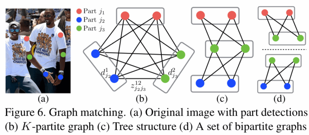
In this collaboration between Saudi and Chinese researchers, the authors use a GAN to detect and upscale very small faces on photographs of large crowds. Even just detecting small faces is an interesting problem that regular face detectors (that appear, e.g., in our previous post) usually fail to solve. And here the authors propose an end-to-end pipeline to extract faces and then apply a generative model to upscale it up to 4x (a process known as superresolution). Here is the pipeline overview from the paper:
Conditional GANs are already widely used for image manipulation; we have mentioned superresolution, but GANs also succeed for style transfer. With GANs, one can learn salient features that correspond to specific image elements — and then change them! In this work, researchers from Princeton, Berkeley and Adobe present a framework for makeup modification on photos. One interesting part of this work is that the authors train separate generators for different facial components (eyes, lips, skin) and apply them separately, extracting facial components with a different network:
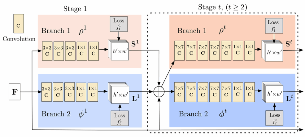
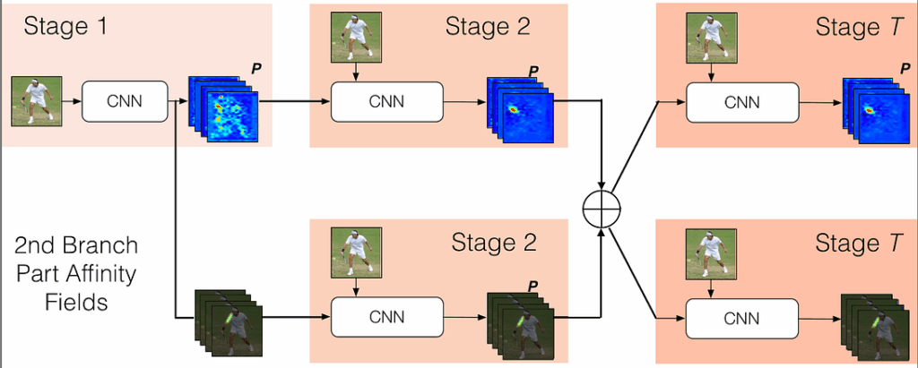
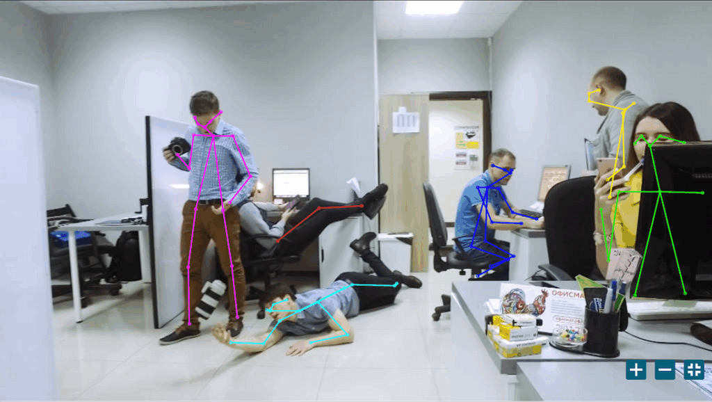
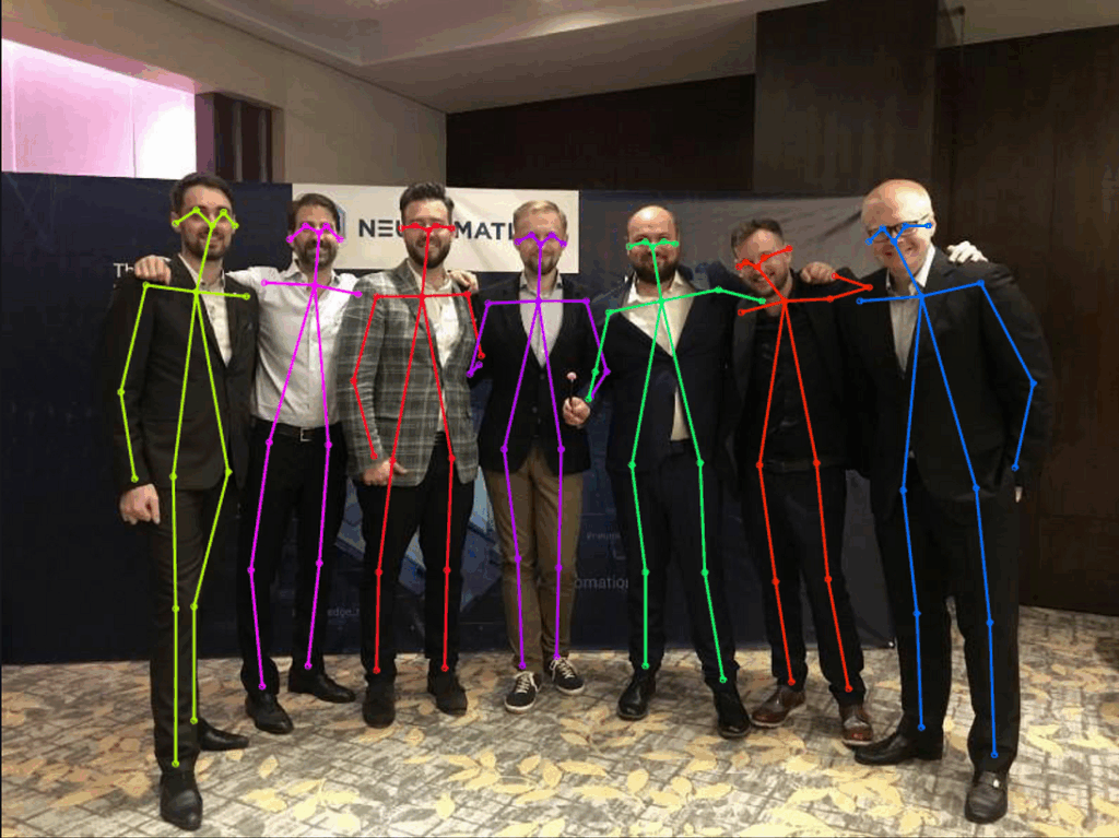
We have already written about pose estimation in the past. One very important subset of pose estimation, which usually requires separate models, is hand tracking. The sci-fi staple of manipulating computers by waving your hands is yet to be fully realized and still requires specialized hardware such as Kinect. As usual, one of the main problems is data: where can you find real video streams of hands labeled in 3D?.. In this work, the authors present a conditional GAN architecture that is able to convert synthetic 3D models of hands to photorealistic images that are then used to train the hand tracking network. This work is very close to our heart as synthetic data is the main emphasis of our studies at Neuromation, so we will likely consider it in more detail later. Meanwhile, here is the “synthetic-to-real” GAN architecture:
Person re-identification (ReID) is the problem of finding the same person on different photos taken in varying conditions and under varying circumstances. This problem has, naturally, been the subject of many studies, and it is relatively well understood by now, but the domain gap problem still remains: different datasets with images of people still have very different conditions (lighting, background etc.), and networks trained on one dataset lose a lot in the transfer to another dataset (and also to, say, a real world application). The picture above shows what different datasets look like. To solve this problem, this work proposes a GAN architecture able to transfer images from one “dataset style” to another, again using GANs to augment real data with complex transformations. It works like this:
This work from the Rensselaer Polytechnic Institute attacks a very specific problem: generating images of human eyes. This is important not only to make beautiful eyes in generated images but also, again, to use generated eyes to work backwards and solve the gaze estimation problem: what is a person looking at? This would pave the way to truly sci-fi interfaces… but that’s still in the future, and at present even synthetic eye generation is a very hard problem. The authors present a complex probabilistic model of eye shape synthesis and propose a GAN architecture to generate eyes according to this model — with great success!
This work from Adobe Research and University of Illinois at Urbana-Champaign is devoted to the very challenging problem of filling in the blanks on an image (see examples above). Usually, inpainting requires understanding of the underlying scene: in the top right on the picture above, you have to know what a face looks like and what kind of face is likely given the hair and neck that we see. In this work, the authors propose a GAN-based approach that can explicitly make use of the features from the surrounding image to improve generation. The architecture consists of two parts, first generating a coarse result and then refining it with another network. And the results are, again, very good:
Well, that’s it for today. This is only part one, and we will certainly continue the CVPR 2018 review in our next installments. See you around!
Sergey Nikolenko Chief Research Officer, Neuromation
Over time, the NeuroNuggets and Neuromation Research series will serve to introduce all AI researchers whom we have collected in our wonderful research team. Today, we are presenting our very own Kaggle master, Alexander Rakhlin! Alexander is a deep learning guru specializing in problems related to medical imaging, which usually means segmentation, object detection, and generally speaking convolutional neural networks, although medical images are often in 3D and are not necessarily RGB images, as we have seen when we discussed imaging mass-spectrometry.
You may have already met Alexander Rakhlin here in our research blog: he has authored a recent post with a general survey of AI applications for healthcare. But today we have great news: Alexander’s paper, Pediatric Bone Age Assessment Using Deep Convolutional Neural Networks (a joint work with Vladimir Iglovikov, Alexander Kalinin, and Alexey Shvets), has been accepted for publication at the 4th Workshop on Deep Learning in Medical Image Analysis (DLMIA 2018)! This is already not the first paper on medical imaging under Neuromation banners, and this is a great occasion to dive into some details of this work. Similar to our previous post on medical concept normalization, this will be a serious and rather involved affair, so get some coffee and join us!
You Are as Old as Your Bones: Bone Age Assessment
Skeletal age, or bone age, is basically how old your bones look like. As a child develops, the bones in his/her skeleton grow and mature; this means that by looking at a child’s bones, you can estimate the average age when a child should have this kind of skeleton and hence learn how old the child is. At this point you’re probably wondering whether this will be a post about archaeology: it’s not often that living children can get an X-ray but nobody knows when they were born.
Well, yes and no. If the child is developing normally, bone age should indeed be roughly within 10% of the chronological age. But there can be exceptions. Some exceptions are harmless but still good to know: e.g., your kid’s growth spurt in adolescence is related to bone age. So if it’s a couple of years more than the chronological age the kid will stop growing earlier, and if the bones are a couple of years “younger” than the rest you can expect a delayed growth spurt. Moreover, given the current height and bone age you can predict the final adult height of a child rather accurately, which can also come in handy: if your kid loves basketball you might be interested whether he’ll grow to be a 7-footer.
Other exceptions are more serious: a significant mismatch between bone age and chronological age can signal all kinds of problems, including growth disorders and endocrine problems. A single reading of skeletal age informs the clinician of the relative maturity of a patient at a particular time, and, integrated with other clinical findings, separates the normal from the relatively advanced or retarded. Successive skeletal age readings indicate the direction of the child’s development and/or show his or her progress under treatment. By assessing skeletal age, a pediatrician can diagnose endocrine and metabolic disorders in child development such as bone dysplasia, or growth deficiency related to nutritional, metabolic, or unknown factors that impair epiphyseal or osseous maturation. In this form of growth retardation, skeletal age and height may be delayed to nearly the same degree, but, with treatment, the potential exists for reaching normal adult height.
Due to all of the above, it is very common for pediatricians to order an X-rays of a child’s hand to estimate his/her bone age… so naturally it’s a great problem to try to automate.
Palm Reading: Assessing Bone Age from the Hand and Wrist
Skeletal maturity is mainly assessed by the degree of development and ossification of secondary ossification centers in the epiphysis. For decades, bone maturity has been usually determined by visual evaluation of the skeletal development of the hand and wrist. Here is what a radiologist looks for when she examines an X-ray of your hand:
The two most common techniques for estimating skeletal age today are Greulich and Pyle and Tanner-Whitehouse (TW2). Both methods use radiographs of the left hand and wrist to assess skeletal maturity based on recognizing maturity indicators, i.e., changes in the radiographic appearance of the epiphyses of tubular bones from the earliest stages of ossification until they fuse with the diaphysis, or changes in flat bones until they reach adult shape… don’t worry, we hadn’t heard these words before either. Let’s show them on a picture:
Conventional techniques for assessing skeletal maturity, such as GP or TW2, are tedious, time consuming, to a certain extent subjective, and even senior radiologists don’t always agree on the results. Therefore, it is very tempting to use computer-aided diagnostic systems to improve the accuracy of bone age assessment, increase reproducibility and efficiency of clinicians.
Recently, approaches based on deep learning have demonstrated performance improvements over conventional machine learning methods for many problems in biomedicine. In the domain of medical imaging, convolutional neural networks (CNN) have been successfully used for diabetic retinopathy screening, breast cancer histology image analysis, bone disease prediction, and many other problems; see our previous post for a survey of these and other applications.
So naturally we tried to apply modern deep neural architectures to bone age assessment as well. Below we describe a fully automated deep learning approach to the problem of bone age assessment using the data from the Pediatric Bone Age Challenge organized by the Radiological Society of North America (RSNA). While achieving as high accuracy as possible is a primary goal, our system was also designed to stay robust against insufficient quality and diversity of radiographs produced on different hardware by various medical centers.
Data
The dataset was made available by the Radiological Society of North America (RSNA), who organized the Pediatric Bone Age Challenge 2017. The radiographs have been obtained from Stanford Children’s Hospital and Colorado Children’s Hospital; they have been taken on different hardware at different times and under different conditions. These images had been interpreted by professional pediatric radiologists who documented skeletal age in the radiology report based on a visual comparison to Greulich and Pyle’s Radiographic Atlas of Skeletal Development of the Hand and Wrist. Bone age designations were extracted by the organizing committee automatically from radiology reports and were used as the ground truth for training the model.
Radiographs vary in scale, orientation, exposure, and often feature specific markings. The entire RSNA dataset contained 12,611 training, 1,425 validation, and 200 test images. Since the test dataset is obviously too small, and its labels were unknown at development time, we tested the model on 1000 radiographs from the training set which we withheld from training.
The training data contained 5,778 female and 6,833 male radiographs. The age varied from 1 to 228 months, the subjects were mostly children from 5 to 15 years old:
Preprocessing I: Segmentation and Contrast
One of the key contributions of our work is a rigorous preprocessing pipeline. To prevent the model from learning false associations with image artifacts, we first remove the background by segmenting the hand.
For image segmentation we use the U-Net deep architecture. Since its development in 2015, U-Net has become a staple of segmentation tasks. It consists of a contracting path to capture context and a symmetric expanding path that enables precise localization; since this is not the main topic of this post, we will just show the architecture and refer to the original paper for details:
We also used batch normalization to improve convergence during training. In our algorithms, we use the generalized loss function
where His the standard binary cross entropy loss function
where
true value of the pixel
is the predicted probability for the pixel, and
is a differentiable generalization of the Jaccard index:
We finalize the segmentation step by removing small extraneous connected components and equalizing the contrast. Here is an how our preprocessing pipeline works:
As you can see, the quality and contrast of the radiograph does indeed improve significantly. One could stop here and train a standard convolutional neural network for classification/regression, augmenting the training set with our preprocessing and standard techniques such as scaling and rotations. We gave this approach a try, and the result, although not as accurate as our final model, was quite satisfactory.
However, original GP and TW methods focus on specific hand bones, including phalanges, metacarpal and carpal bones. We decided to try to use this information and train separate models on several specific regions in high resolution to numerically evaluate and compare their performance. To correctly locate these regions, we have to transform all images to the same size and position, i.e., to bring them all to the same coordinate space, a process known as image registration.
Preprocessing II: Image Registration with Key Points
Our plan for image registration is simple: we need to detect the coordinates of several characteristic points in the hand. Then we will be able to compute affine transformation parameters (zoom, rotation, translation, and mirroring) to fit the image into the standard position.
To create a training set for the key points model, we manually labelled 800 radiographs using VGG Image Annotator (VIA). We chose three characteristic points: the tip of the distal phalanx of the third finger, tip of the distal phalanx of the thumb, and center of the capitate. Pixel coordinates of key points serve as training targets for our regression model.
The key points model is, again, implemented as a deep convolutional neural network, inspired by a popular VGG family of models but with regression output. The VGG module consists of two convolutional layers with Exponential Linear Unit activation, batch normalization, and max pooling. Here is the architecture:
The model is trained with Mean Squared Error loss (MSE) and Adam optimizer:
To improve generalization, we applied standard augmentations to the input. including rotation, translation and zoom. The model outputs 6 coordinates, 2 for each of the 3 key points.
Having found the key points, we calculate affine transformations (zoom, rotation, translation) for all radiographs. Our goal is to keep the aspect ratio of an image but fit it into a uniform position such that for every radiograph:
the tip of the middle finger is aligned horizontally and positioned approximately 100 pixels below the top edge of the image;
the capitate is aligned horizontally and positioned approximately 480 pixels above the bottom edge of the image.
By convention, bone age assessment uses radiographs of the left hand, but sometimes images in the dataset get mirrored. To detect these images and adjust them appropriately, we used the key point for the thumb.
Let’s see a sample of how our image registration model works. As you can see, the hand has been successfully rotated into our preferred standard position:
And here are some more examples of the entire preprocessing pipeline. Results of segmentation, normalization and registration are shown in the fourth row:
Bone age assessment models
Following Gilsanz and Ratib’s Hand Bone Age: a Digital Atlas of Skeletal Maturity, we have selected three specific regions from registered radiographs and trained an individual model for each region:
whole hand;
carpal bones;
metacarpals and proximal phalanges.
Here are the regions and some sample corresponding segments of real radiographs:
Convolutional neural networks are typically used for classification tasks, but bone age assessment is a regression problem by nature: we have to predict age, a continuous variable. Therefore, we wanted to compare two settings of the CNN architecture, regression and classification, so we implemented both. The models share similar parameters and training protocols, and only differ in the two final layers.
Our first model is a custom VGG-style architecture with regression output. The network consists of a stack of six convolutional blocks with 32, 64, 128, 128, 256, 384 filters followed by two fully connected layers of 2048 neurons each and a single output (we will show the picture below). The input size varies depending on the considered region of an image. For better generalization, we apply dropout layers before fully connected layers. We rescale the regression target, i.e., bone age, to the range [−1, 1]. To avoid overfitting, we use train time augmentation with zoom, rotation and shift. The network is trained with the Adam optimizer by minimizing the Mean Absolute Error (MAE):
The second model, for classification, is very similar to the regression one except for the two final layers. One major difference is a distinct class assigned to each bone age. In the dataset, bone age is expressed in months, so we considered all 240 classes, and the penultimate layer becomes a softmax layer with 240 outputs. This layer outputs vector of probabilities, where probability of a class takes a real value in the range [0, 1]. In the final layer, the probabilities vector is multiplied by a vector of distinct bone ages [1, …, 239, 240]. Thereby, the model outputs a single expected value of the bone age. We train this model using the same protocol as the regression model.
Here is the model architecture for classification; the regression model is the same except for the lack of softmax and binning layers:
Results
We evaluated the models on a validation set of 1000 radiographs withheld from training. Following GP and TW methods that account for sex, for each spatial zone we trained gender-specific models separately for females and males, and compared them to a gender-agnostic model trained on the entire population. Here is a summary of our results which we will then discuss:
It turns out that adding gender to the input significantly improves accuracy, by 1.4 months on average. The leftmost column represents the performance of a regression model for both genders. The region of metacarpals and proximal phalanges (region C) has Mean Absolute Error (MAE) 8.42 months, while MAE of the whole hand (region A) is 8.08 months. A linear ensemble of the three zones improves overall accuracy to 7.52 months (bottom row in the table).
Gender-specific classification models (fourth and fifth columns) perform slightly better than regression models and demonstrate a MAE of 6.16 and 6.39 months respectively (bottom row)
Finally, in the sixth column we show an ensemble of all gender-specific models (classification and regression). On the validation dataset it achieved state of the art accuracy of 6.10 months, which is a great result both in terms of the bone age assessment challenge and from the point of view of real applications.
Conclusion
Let’s wrap up: in this post, we have shown how to develop an automated bone age assessment system that can assess skeletal maturity with remarkable accuracy, similar to or better than an expert radiologist. We have numerically evaluated different zones of a hand and found that bone age assessment could be done just for metacarpals and proximal phalanges without significant loss of accuracy. To overcome the widely ranging quality and diversity of the radiographs, we introduced rigorous cleaning and standardization procedures that significantly increased robustness and accuracy of the model.
Our model has a great potential for deployment in clinical settings to help clinicians in making bone age assessment decisions accurately and in real time, even in hard-to-reach areas. This would ensure timely diagnosis and treatment of growth disorders in their little patients. And this is, again, just one example of what the Neuromation team is capable of. Join us later for more installments of Neuromation Research!
Alexander Rakhlin Researcher, Neuromation
Sergey Nikolenko Chief Research Officer, Neuromation
Neuromation researchers are attending ICML 2018, one of the two largest and most important conferences in machine learning (the other one is NIPS, and we hope to get there as well). Here is a part of our team together with our long-term friends and collaborators from Insilico Medicine next to their booth:
Left to right: Kyryl Truskovsky (Lead Researcher, Neuromation), Rauf Kurbanov (Lead Researcher, Neuromation), Alexander Aliper (President of EMEA, Insilico Medicine), Alex Zhavoronkov (CEO, Insilico Medicine), Denys Popov (CIO, Neuromation), Ira Opanasiuk (HR Director, Neuromation).
Neuromation and Insilico Medicine are collaborating in the many areas of high-performance computing and deep learning; see, e.g., this previous post on one topic of our collaboration. In the area of blockchain technology, Neuromation has partnered with Longenesis, which is a partnership between Insilico Medicine and the BitFury Group.
Both our teams share passion for using the latest advances in artificial intelligence, high-performance computing and blockchain for healthcare. We are happy to be a part of the vibrant ecosystem of companies in this space which resembles the early days of the Internet. And we are building the Internet of Health.
We are looking forward to further collaboration with Insilico and to many other collaborations that ICML can bring. Deep learning galore!
Although computer vision is our main focus, here at Neuromation we are pursuing all aspects of deep learning. Today, it is my great pleasure to introduce Elena Tutubalina, Ph.D., our researcher from Kazan who specializes on natural language processing. She has joined Neuromation part-time to work on a very interesting project related to sentiment analysis and named entity recognition… but this is a story for another day.
Presented at a NAACL workshop before the journal version, our paper was. Elena’s photo from the NAACL 2018 social event, we show to you:
The Adverse Effects of Social Networks
Nowadays it is hard to find a person who has no social media account in at least one social network, usually more. And it’s virtually impossible to find a person who has never heard about one. This unprecedented popularity of social networks, and the huge amount of stuff people put on their pages, means that there is an enormous quantity of data available in social networks on almost any topic. This data, of course, is nothing like a top quality research report, but there are tons of opinions of real people on all kinds of subjects, and it would be strange to forgo this wisdom of the crowds.
To explain what exactly we will be looking for, let us take a break from social media (exactly as the doctors order, by the way) and look a little bit back on history. One of the most important topics in human history has always been human health. It was important in ancient Egypt, Greece, or China, in Napoleon’s France or modern Britain. Medicine invariably comes together with civilization, and with medicine come the drugs, starting from a shaman’s herbs and all the way to contemporary medicaments.
Unfortunately, with drugs come side effects. Сocaine, for example, was famously introduced as a cough stopper, and back in the good old days cocaine was given to kids (no kidding) and Coca-Cola stopped using fresh coca leaves with significant amounts of cocaine only by 1903. Modern medications also can have side effects (including sleep eating, gambling urges, or males growing boobs), but these days we at least try to test for side effects and warn about them.
To reveal the side effects, drug companies conduct long and costly clinical trials. It takes literally years for a drug to become accepted as a safe one, and while in principle it’s a good thing to test thoroughly in reality it means that many people die from potentially curable diseases while the drugs are still under testing. But even this often overly lengthy process does not catch all possible side effects, or, as they are usually called in scientific literature, adverse drug reactions (ADR): people are too diverse to make a representative group of all possible patient conditions and drug interactions. And this is where social media can help.
Once the drug is released, and people are actually using it, they (unfortunately) can have side effects, including unpredictable side effects like a weird combination of three different drugs that no one could have tested for. But once it happens, people are likely to rant about it on social media, and we could collect that data and use it. By the way, it would be an oversimplification to think that side effects could only be negative. Somewhat surprisingly, it is not that rare when a drug initially targeted to cure one disease is found to be a cure for some completely unrelated condition; kind of like cocaine proved to be so much more than a cough syrup. So the social media data is actually a treasure trove of information ready to be scrapped.
And this is exactly what our paper is about: looking for adverse drug effects in social media. Let’s dive into the details…
The Data and the Problems
To be more precise, the specific dataset that we have used in the paper comes from Twitter. In natural language processing, it is really common to scrape Twitter since it is open, popular, and the texts are so short that we can assume that each tweet stays on a single topic. All of these characteristics are important, by the way: the problems of handling personal data are by now a subject of real importance, especially in such a delicate sphere as healthcare, and we don’t want to break someone’s privacy.
At this point, it might seem that once we have the data it is a simple matter of keyword search to find the drug names and the corresponding side effects: if the same tweet mentions both “cocaine” and “muscle spasm” it is quite likely that muscle spasms are a side effect of cocaine. Unfortunately, it’s not that simple: we can’t expect a random guy snorting cocaine on Twitter to use formal medical language to describe his or her symptoms. People on Twitter (and more broadly in social media) do not use medical terminology. To be honest, we can consider ourselves lucky if they use the actual name of the drug at all; we all know how tricky these drug names can be.
Thus, in the context of mining social media we have to translate a text written in “social media language” (e.g., “I can’t fall asleep all night” or “head spinning a little”) to “formal medical language” (e.g., “insomnia” and “dizziness” respectively). Sometimes the examples are even less obvious:
And so on, and so forth. You can seehow this goes beyond simple matching of natural language expressions and vocabulary elements: string matching approaches cannot link social media language to medical concepts since the words often do not overlap at all. We call the task of mapping everyday language to medical terminology medical concept normalization. If we solve this task, we can bridge the gap between the language of Twitter and medical professionals.
Natural Languages and Recurrent Neural Networks
OK, suppose we do have the data in the form of a nicely scraped and parsed set of tweets. Now what? Now it is most important part: we need to process this data, mining it for something that could sound like an adverse drug effect. So how on Earth can a model guess that “I can’t fall asleep all night” is actually about “insomnia”? There is not a single syllable in common between these two phrases.
The answer, as usual in our series, comes from neural networks. Modern state of the art natural language processing often uses neural networks, to be more precise, a special kind of them called recurrent neural networks (RNNs). An RNN can work with sequence data, keeping some intermediate information inside, in its hidden state, to “remember” previous parts of the sequence. Language is a perfect example of sequential data: it is a string of… well, something; some models work with words, some go down to the level of characters, some combine words into bigrams, but in any case the input is a discrete sequence.
We will not go into the details of recurrent neural networks; maybe in a next post. Let us just show the network architecture that we used in this paper:
In the upper left part of you can see a recurrent neural network. It is receiving as input a sequence of words (previously processed into embeddings, another interesting idea that we will explain some other time). The network receives a word and outputs a vector a, but also at the same time sends some information to its “future self”, to the next timestep. This piece of information is called a hidden state, denoted on the figure as h, and formally it is also simply a vector of numbers. Another interesting part is that the sequence is actually handled in two directions: from start to end and vice versa; such a setup is called a bidirectional RNN.
On the right side of the figure you can see a bubble labeled “Softmax”. This is a standard final layer for classification: it turns a vector of extracted features into probabilities of discrete classes. Basically, every neural network that solves a classification problem has a softmax layer in the end, which means that the entire network serves as a feature extractor, and the features are then fed into a logistic regression. In this case, softmax outputs the probabilities of medical terms from a specific vocabulary.
This is all very standard stuff for modern neural networks. The interesting part of the figure is at the bottom. There, we extract additional semantic similarity features that are fed into the softmax layer separately. These features result from analysing UMLS, the largest medical terminological system that links terms and codes between your doctor, your pharmacy, and your insurance company. This system integrates a wide range of terminology in multiple domains: more than 11 million terms from over 133 English source vocabularies into 3.6 million medical concepts. Besides English, UMLS also contains source vocabularies in 24 other languages.
So do these features help? What do the results look like, anyway? Let’s find out.
Our Results
Here is an example of how our system actually works in practice:
The model takes a post from social media (a tweet, like on the picture, or any other text) as input and maps it to a number of standard medical terms. As you can see, some of the concepts are relatively straightforward (“lousy sleeping” produced “difficulty sleeping”) but some, like “asthenia”, do not share any words with the original.
We evaluated our model with 5-fold cross-validation on a publicly available AskAPatient dataset LINK2. This dataset consists of gold-standard mappings of social media messages and medical concepts from a CSIRO adverse drug event corpus LINK3. Our results are for CADEC dataset, which consists of posts from AskAPatient forum annotated by volunteers. Since the volunteers did not have to have any medical training, and they could be inaccurate in some cases (even after detailed instructions), their answers were proof-read by experts in the field, including a pharmacist. The dataset contains adverse drug reactions (ADRs) for 12 well-known drugs, like Diclofenac.
We’ll let the numbers speak for themselves:
Colored bars always look convincing; but what do they stand for? We compare our system with three standard architectures. The RNN and CNN labels should be familiar to our readers: we have briefly touches upon RNNs in this post and have explained CNNs for quite a few posts in the past (see, e.g., here). We will not go into the details of what exact convolutional architectures we used for comparison, let’s just say that one-dimensional convolutions are also a very common tool in natural language processing, and we used the architectures shown in a 2016 paper on this subject by researchers from Oxford.
DNorm is the previous best result for this task, the so-called state of the art, from the era before the deep learning revolution. This model comes from a 2013 paper by researchers from the National Center for Biotechnology Information, and it illustrates very well just how amazing the deep learning revolution has been. This result is only 5 years old, it required the best tricks in business, and it is already hopelessly outmatched even by relatively straightforward neural network architectures, and further improved in our work: we have an error rate of 14.5% compared to their 26.5%, almost half their error rate!
Let us summarize. Improvements in social media mining provided by deep learning can help push this field (dubbed pharmacovigilance, a buzzword on the rise) from experiments to real life applications. That’s what these numbers are for: you can’t solve a problem like this perfectly without strong AI, but when you have an error rate of 25% it doesn’t work at all, and when you push it down to 15%, then 10%, then 5%… at some point the benefits begin to outweigh the costs. By faster and more accurate analysis of the people’s input on the drugs they use, we hope to eventually help pharmaceutical companies to reduce side effects of the drugs they produce. This is yet another example of how neural networks can be changing our lives to the better, and we are happy to be part of this process.
Elena Tutubalina Researcher, Neuromation
Sergey Nikolenko Chief Research Officer, Neuromation
Deep learning is hot. There are lots of projects on the cutting edge of deep learning appearing every month, lots of research papers on deep learning coming out every week, and lots of very interesting models for all possible applications being developed and trained every day.
With this neverending stream of constant advances, it is common that when you are just about to start solving some computer vision (or natural language processing, or any other) problem, you naturally begin by googling possible solutions, and there is always a bunch of open repositories with ready-made models that promise to solve all your problems. If you are lucky enough, you will even find some pre-trained weights for these neural network models, and even maybe a handy API for them. Basically, for most problems you can usually find a model, or two, or a dozen, and all of them seem to work fine.
So if that is the case, what exactly are we doing here? Are deep learning experts just running existing ready-made models (when they are not doing state of the art research where these models actually come from)? Why the big bucks? Well, actually applying even ready-to-use products is not always easy. In this post, we will see a specific example of why it is hard, how to detect the problem, and what to do when you noticed it. We have written this post together with our St. Petersburg researcher Anastasia Gaydashenko, whom we have already presented in a previous post on segmentation; she has also prepared the models that we use in this post.
And we will be talking about cows.
Problem description
We begin with the problem. It is quite easy to formulate: we would like to learn to track objects from flying drones. We have already talked about very similar problems: object detection, segmentation, pose estimation, and so on. Tracking is basically object detection but for videos rather than still images. Performance is also very important because you probably want tracking to be done in real time: if you spend more time to process the video than to record it you cut off most possible applications that require raising alarms or round-the-clock tracking. And today, we will consider tracking with a slightly unusual but very interesting example.
We at Neuromation believe that artificial intelligence is the future of agriculture. We have written about it extensively, and we hope to bring the latest advances of computer vision and deep learning in general to agricultural applications. We are already applying computer vision computer vision models to help grow healthy pigs, by tracking them in the Piglet’s Big Brother project. So as the testing grounds for the models, we chose this beautiful video, Herding Cattle with a Drone by Trey Lyda for La Escalera Ranch:
We believe that adding high-quality real-time tracking from drones that herd cows opens up even more opportunities: maybe some cows didn’t pay attention to the drone and were left behind, maybe some of them got sick and can’t move as fast or at all… the first step to fixing these problems would be to detect them. And it appears that there are plenty of already developed solutions for tracking that should work for this problem. Let’s see how they do…
Simple Online and Realtime Tracking
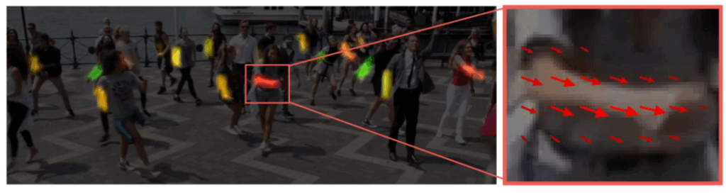
The most popular and one of the simplest algorithms for tracking is SORT (Simple Online and Realtime Tracking). It can track multiple objects in real time but the algorithm merely associates already detected objects across different frames based on the coordinates of detection results, like this:
The idea is to use some off-the-shelf model for object detection (we already did a survey of those here) and then plug the results into the SORT algorithm that matches detected objects across frames.
This approach obviously yields a multi-purpose algorithm: SORT doesn’t need to know which type of object we track. It doesn’t even need to learn anything: to perform the associations SORT uses mathematical heuristics such as maximizing the IOU (intersection-over-union) metrics between bounding boxes in neighboring frames. Each box is labeled with a number (object id), and if there is no relevant box in the next frame, the algorithm assumes that the object has left the frame.
The quality of such an approach naturally depends a lot on the quality of the underlying object detection. The whole point of the original SORT paper was to show that object detection algorithms have advanced so much that you don’t have to do anything too fancy about tracking and can achieve state-of-the-art results with straightforward heuristics. Since then, improvements have appeared, in particular the next generation of the SORT algorithm, Deep SORT (deep learning is really fast: SORT came out in 2016, and Deep SORT already in 2017). It was designed especially to reduce the number of switchings between identities, ensuring that the tracking is more stable.
First results
To use SORT for tracking, we need to plug in some model for the detection step. In our case, it could be any object detection model pretrained to recognize cows. We used this open repository that includes a SORT implementation based on YOLO (actually, YOLOv2) detection model; it also has an implementation of Deep SORT.
Since YOLO is pretrained on the standard COCO dataset that has “cow” as one of its classes, we can simply launch the detection and tracking. The results are quite poor:
Note that we haven’t made any bad decisions along the way. Frankly, we haven’t really made any decisions at all: we are using a standard pretrained implementation of SORT with a standard YOLO model for object detection that usually works quite well. But the video clearly shows that the results are poor because of the first step, detection. In almost all frames the model does not detect any cows, only sometimes finding a couple of them. So we need to go deeper…
You Only Look Once
To understand the issue and decide how to deal with it, let’s take a closer look at the YOLO architecture.
The pipeline itself is pretty straightforward: unlike many popular detection models which perform detection on many region proposals (RoIs, region of interest), YOLO passes the image through the neural network only once (this is where the title comes from: You Only Look Once) and returns bounding boxes and class probabilities for predictions. Like this:
To do that, YOLO breaks up the image into a grid, and for each cell in the grid considers a number of possible bounding boxes; neural networks are used to estimate the confidence that each of those boxes contains an object and find class probabilities for this object:
The network architecture is pretty simple too; it contains 24 convolutional layers followed by two fully connected layers, reminiscent of AlexNet and even earlier convolutional architectures:
Since the original image is divided into cells, detection happens if the center of an object falls into a cell. But since each grid cell only predicts two boxes, the model struggles with small objects that appear in groups, such as a flock of birds… or a herd of cows (or is it a kine? a flink? it’s all pure rubbish, of course). It is even explicitly pointed out by the authors in the section on the limitations of their approach.
Okay, so by now we have tried a straightforward approach that seemed very plausible but utterly failed. Time to pivot.
Pivoting to a different model
As we have seen, even if you can find open repositories that seem tailor-made for your specific problem, the models you find, even if they are perfectly good models in general, may not be the best option for your particular problem.
To get the best performance (or some reasonable performance, at least), you usually have to try several different approaches. So as the next step, we changed the model to Mask R-CNN that we have talked about in detail in one of our previous posts. Due to a totally different approach to detection, it should be able to recognize cows better, and it really did:
The basic network that you can download from the repositories was also trained on the COCO dataset.
But to achieve even better results, we decided to get rid of all extra classes and train the model only on classes responsible for cows and sheep. We left sheep in because, first, we wanted to reproduce the results on sheep as well, and second, they look pretty similar from afar, so a similar but different class could be useful for the detection.
There is a pretty easy way to upload new training data for the model in the Mask R-CNN repository that we used. So we retrained the network to detect only these two classes. After that, all we needed to do was to embed the new detection model into the tracking algorithm. And here we go, the results are now much better:
We can again compare all three detection versions on a sample frame from the video.
YOLO did not detect anything:
Vanilla Mask R-CNN did much better but it’s still not something you can call a good result:
And our version of Mask R-CNN is better yet:
All the code for our experiments can be found here, in the Neuromation fork of the “Tracking with darkflow” repository.
As you can see, even almost without any new code, by fiddling with existing repositories you can often go from a completely unworkable model to a reasonably good one. Still, even in the last picture one can notice a few missing detections that really should be there, and the tracking based on this detector is also far from perfect yet. Our simple illustration ends here, but the real work of artificial intelligence experts only begins: now we have to push the model from “reasonable” to “truly useful”. And that’s a completely different flink of cows altogether…
Sergey Nikolenko Chief Research Officer, Neuromation
We have great news: we’ve got not one, not two, but three papers accepted to the DeepGlobe workshop at the top computer vision conference, CVPR 2018! This is a big result for us: it shows that our team is able to compete with the very best and get to the main conferences in our field.
Today, we present one of the solutions that got accepted, and it is my great pleasure to present the driving force behind this solution, one of our deep learning researchers in St. Petersburg, with whom we have co-authored this post. Please meet Sergey Golovanov, an experienced competitive data scientist whose skills have been instrumental for the DeepGlobe challenge:
Sergey Golovanov Researcher, Neuromation
The DeepGlobe Challenge
Satellite imagery is a treasure trove of data that can yield many exciting new applications in the nearest future. Over the last decades, dozens of satellites from various agencies such as NASA, ESA, or DigitalGlobe that sponsored this competition, have collected terabytes upon terabytes of data.
At the same time, satellite imagery has not yet become the target of much research in computer vision and deep learning. There are few large-scale publicly available datasets, and data labeling is always a bottleneck for segmentation tasks. The DeepGlobe Challenge is designed to bridge this gap, bringing high-quality and at the same time labeled satellite imagery to everyone; see this paper by DeepGlobe organizers for a more detailed description of the dataset.
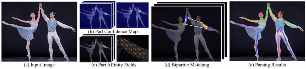
By virtue of data science competitions, organizers try to draw the attention of AI researchers and practitioners to specific problems or whole problem domains and thereby spur the development of new models and algorithms in this field. To attract the deep learning community to analyzing satellite imagery, DeepGlobe presented three tracks with different tasks highly relevant for satellite image processing: road extraction, building detection, and land cover classification. Here are three samples of labeled data for these tasks:
All of these tasks are formulated as semantic segmentation problems; we have already written about segmentation problems before but will also include a reminder below.
A part of our team from the Neuromation Labs at St. Petersburg, Russia, took part in two of the three tracks: building detection and land cover classification. We took the third place in building detection and fourth and fifth places in land cover classification (see the leaderboard) and got three papers accepted for the workshop! In this post, we will explain in detail the solution that we prepared for the building detection track.
Semantic segmentation
Before delving into the details of our solution, let us first discuss the problem setting itself. Semantic segmentation of an image is a partitioning of the image into separate groups of pixels, areas corresponding to certain objects, and at the same time classifying what is the type of object in every area (see also our previous post on this subject). That is, the problem looks something like this:
Deep Learning for Segmentation: Basic Architecture
We have spoken about convolutional neural networks and characteristics of convolutions many times in our previous posts (for example, see here, here or here), so we will not discuss them in too many details and will go straight to the architectures.
The most popular and one of the most effective neural network architectures for semantic segmentation is U-Net and its extensions (there are plenty of modifications, which is always a good sign for the basic architecture as well). The architecture itself consists of an encoder and a decoder; as you can see in the figure below, U-Net is very aptly named:
The encoder creates compressed image representations (feature maps), extracting multiscale features and thereby implicitly taking into account local context information within certain neighborhoods on the image. Real life problems often have not too much labeled data, so usually encoders in U-Net and similar architectures use transfer learning, that is, use a classifier pre-trained on ImageNet without the last layer of classification (i.e., only with convolutional layers) as the encoder. Actually, this is useful even if data is plentiful: this usually increases the rate of convergence of the model and improves segmentation results, even in domains that do not overlap with ImageNet such as segmentation of cell nuclei or, in our case, satellite imagery.
The decoder takes as input the feature maps obtained from the encoder and constructs a segmentation map, gradually increasing the resolution for more accurate localization of object boundaries. The main novel feature of U-Net that gives the architecture its form and name are the skip-connections that let the decoder “peek” into intermediate, higher-resolution representations from the encoder, combining them with the outputs of the corresponding level of the decoder. Otherwise, a decoder in U-Net is usually just a few layers of convolutions and deconvolutions.
Deep Learning for Segmentation: Loss Functions
There is one more interesting remark about segmentation as a machine learning problem. On the surface, it looks like a classification problem: you have to set a class for every pixel in the image. However, if you treat it simply as a classification problem (i.e., start using per-pixel cross-entropy as the objective function to optimize the model) it won’t work too well.
The problem with this approach is that it does not capture the spatial connections between the pixels: classification problems are independent for every pixel, and the objective function has no idea that a single pixel in the middle of the sea cannot really be a lawn even if it turns out to be green. This will lead to small holes appearing on segmentation results and very complicated boundaries between different classes.
To solve this problem, we have to balance the standard cross-entropy with some other loss function which is developed specifically for segmentation. We won’t go into the mathematical details here, but the 2017 approach here has been to add the average DICE loss which allows to optimize the value of IoU (Intersection over Union). However, in order to strike the right balance for clear boundaries and absence of holes, one has to to choose the coefficients between these two losses very carefully.
The 2018 approach, rapidly growing in popularity, is the Lovász-Softmax loss (and a similar Lovász-Hinge loss), which serves as a differentiable surrogate for intersection-over-union. We have also used the Lovász-Softmax loss in another DeepGlobe paper of ours, devoted to the land cover classification challenge, so we will concentrate on the architectures here and perhaps return to discuss the loss functions in a later post. In any case, our experiments on this challenge have also shown that both DICE and Lovász-Softmax losses give tangible increases in segmentation quality.
Deep Learning for Segmentation: Beyond the Basics
There are plenty of architectures based on the principles described above; see, e.g., this repository of links on semantic segmentation. But we would like to pay special attention to two very interesting ideas that have already proven to be very effective in practice: Atrous Spatial Pyramid Pooling with Image Pooling and ResNeXt-FPN.
The basic idea of the first approach is to use several parallel atrous convolutions (dilated convolutions) and image pooling at the end of the encoder, which are eventually combined through a 1×1 convolution. An atrousconvolution is a convolution where there is some distance between the elements of the kernel, called rate, like here:
Image pooling simply means averaging over the entire feature map. This architecture effectively extracts multiscale features and then uses their combination to actually produce the segmentation. In this case, the encoder is made shallow, with a finite size of the feature maps, 8 or 16 times smaller than the input image size:
This leads to feature maps of higher resolution. A good rule of thumb here is to use as simple a decoder as possible since each layer of the decoder is only required to increase the image resolution by a factor of two, and thanks to the U-Net architecture and spatial pyramid pooling it has quite a lot of input information to do it.
ResNeXt-FPN is basically the Feature Pyramid Network model with ResNeXt, a modern architecture commonly used for object detection (for example, in Faster-RCNN), but adapted for segmentation. Again, the architecture consists of an encoder and a decoder. However, now for segmentation we use feature maps from each decoder level, not just from the last layer with highest resolution.
Since these maps have different sizes, they are resized (to match the largest) and then combined together:
This architecture has long been known to work very well for segmentation, taking first place in the COCO 2017 Stuff Segmentation Task.
DeepGlobe Building Detection Challenge
The task in the Building Detection Challenge is, rather surprisingly, to detect buildings. At this point an astute reader might wonder why we need to solve this problem at all. After all, there are a lot of cartographic services where these buildings are already labeled. In the world where you can go to Google Maps and find your city mapped out to the last detail, how is building detection a challenge?
Well, the astute reader would be wrong. Yes, such services exist, but usually they label buildings manually. First of all, this means that labeling costs a lot of money, and cartographic services run into the main bottleneck of modern AI: they need lots of real data that can be produced only by manual labeling.
Moreover, this is not a one-time cost: you cannot label the map of the world once and forget about it. New buildings are constructed all the time, and old ones are demolished. Satellites keep circling the Earth and producing their images pretty automatically, but who will keep re-labeling them? A high-quality detector would help solve these problems.
But cartography is not the only place where such a detector would be useful. Analysis of urbanization in an area, which relies on the location of the buildings, could be useful for realtor, construction, and insurance companies, and, in fact, ordinary people. Another striking application of building detection, one of the most important in our opinion, is disaster relief: when one needs to find and evaluate destructed buildings as fast as possible to save lives, any kind of automation is priceless.
Let us now go back to the challenge. Satellite images were selected from the SpaceNet dataset provided by DigitalGlobe. Images have 30cm per pixel resolution (which is actually a pretty high resolution when you think about it) and have been gathered by the WorldView-3 satellite. The organizers chose several cities — Las Vegas, Paris, Shanghai, and Khartoum — for the challenge. Apart from color photographs (which means three channels for the standard RGB color model), SpaceNet also contains eight additional spectral channels which we will not go into; suffice it to say that satellite imagery contains much, much more than meets the eye.
How does one evaluate the quality of a detector? For evaluation, the organizers proposed to use the classical F1-score:
Here TP (true positive) is the number of correctly detected polygons of buildings, N is the number of existing real building polygons (unique for every building), and M is the number of buildings in the solution. A building proposal (a polygon produced by the model) is considered to be a true positive if the real building polygon that has the largest IoU (Intersection over Union) with the proposal has IoU greater than 0.5; otherwise the proposal is a false positive.
In our solution for the segmentation of buildings, we used an architecture similar to U-Net. As the encoder, we used the SE-ResNeXt-50 pretrained on ImageNet. We chose it because this classifier is of high enough quality and does not require too much memory, which is important to maintain a large batch size during training.
To the encoder, we added Atrous Spatial Pyramid Pooling with Image Pooling. The decoder also contains four blocks, each of which is a sequence of convolution, deconvolution, and another convolution. Besides, following the U-Net idea we added skip-connections from the encoder at each level of the decoder. The full architecture is shown in the figure below.
With this model, we did our first experiments and looked at the results… only to find that a good architecture is not enough to produce a good result. The main problem was that in many situations, buildings were clustered very close together. This dense placement made it very difficult for the model to distinguish individual buildings: it usually decided to simply lump them all together into one uber-building. And this was very bad for the competition score (and for the model’s results in general) because the score was based on identifying specific buildings rather than classifying pixels.
To fix this problem, we needed to do instance segmentation, i.e., learn to separate instances of the same class in the segmentation map. After trying several ways of separating the buildings, we decided on a simple but quite effective solution: the watershed algorithm. Since the watershed algorithm needs an initial approximation of the instances (in the form of markers), in addition to the binary segmentation mask our neural network also predicted the normalized pixel distance of the building to its boundary (“energy”). The markers were obtained by binarizing this energy with a threshold. In addition, we increased the input size of images by a factor of two, which allowed to construct more precise segmentation.
As we explained above, we used the sum of binary cross-entropy and the Lovász-Hinge loss function as the objective for the binary mask and the mean squared error for energy. The model was trained on 256×256 crops of input RGB images. We used standard augmentation methods: rotations by multiples of 90 degrees, flips, random scaling, changes in brightness and contrast. We sampled images in the batch based on the value of the loss that was observed on them, so that images with larger error would appear in a training batch more often.
Results and conclusion
Et voila! In the end, our solution produced building detection of quite good quality:
These animated GIFs show binary masks of the buildings on the left and predicted energy on the right. Naturally, the current detection, even state of the art models such as this one, is still not perfect and we still have a lot to do, but it appears that this quality is already quite sufficient for industrial use.
Let’s wrap up: we have discussed in detail one of our papers accepted for the DeepGlobe CVPR workshop. There are two more for land cover classification, i.e., for segmenting satellite images into classes like “forest”, “water”, or “rangeland”; maybe we will return to them in a later post. Congratulations to everyone who has worked on these models and papers: Alexander Rakhlin, Alex Davydow, Rauf Kurbanov, and Aleksey Artamonov! We have a great team here at Neuromation Labs, and we are sure there are many more papers, competitions, and industrial solutions to come. We’ll keep you posted.
Sergey Golovanov Researcher, Neuromation
Sergey Nikolenko Chief Research Officer, Neuromation
Today we continue the NeuroNuggets series with a new installment. This is the first time when a post written by one of our deep learning researchers was so long that we had to break it up into two parts. In the first part, we discussed the notion of a computational graph and what functionality should a deep learning framework have; we found out that they are basically automated differentiation libraries and understood the distinction between static and dynamic computational graphs. Today, meet again Oktai Tatanov, our junior researcher in St. Petersburg, who will be presenting a brief survey of different deep learning frameworks, highlighting their differences and explaining our choice:
Comparative popularity
Last time, we finished with this graph published by the famous deep learning researcher Andrej Karpathy; it shows comparative popularity of deep learning frameworks in the academic community (mentions in research papers):
Unique mentions of deep learning frameworks in arXiv papers (full text) over time, based on 43K ML papers over last 6 years. Source
We see that the top 4 general-purpose deep learning frameworks right now are TensorFlow, Caffe, Keras, and PyTorch. Today, we will discuss the similarities and differences between them and help you make the right choice of a framework.
Tensorflow
TensorFlow is probably the most famous deep learning framework; it is being developed and maintained by Google. It is written in C++/Python and provides Python, Java, Go and JavaScript API. TensorFlow uses static computational graphs, although a recently released TensorFlow Fold library has added support for dynamic graphs as well. Also, since version 1.7 TensorFlow took a different step towards dynamic execution and implemented eager execution that can evaluate Python code immediately, without building graphs.
At present, TensorFlow has gathered the largest deep learning community around it, so there are a lot of videos, online courses, tutorials, and so on. It offers support for running models on multiple GPUs and can even split a single computational graph over multiple machines in a computational cluster.
Apart from purely computational features, TensorFlow provides an awesome extension called TensorBoard that can visualize the computational graph, plot quantitative metrics about the execution of model training or inference, and basically provide all sorts of information necessary to debug and fine-tune a deep neural network in an easier way.
Plenty of data scientists consider TensorFlow to be the primary software tool of deep learning, but there are also some problems. Despite the big community, learning is still difficult for beginners, and many experts agree that other mainstream frameworks are faster than TensorFlow.
As an example of implementing а simple neural network, look at the following:
It’s not so elementary for beginners, but it shows the main concepts in TensorFlow, so let us try to focus on the code structure only first. We begin by defining the computational graph: placeholders, variables, operations (maximum, matmul) and the loss function at the end. Then we assign an optimizer that defines what and how we want to optimize. And finally, we train our graph over and over in a special execution environment called a session.
Unfortunately, if you want to improve the network’s architecture with conditionals or loops (this is especially useful, even essential for recurrent neural networks), you cannot simply use python keywords. As you already know, a static graph is constructed and compiled once, so to add nodes to the graph you should use special control flow or higher order operations.
For instance, to add a simple conditional to our previous example, we have to modify the previous code like this:
The Caffe library was originally developed at UC Berkeley; it was written in C++ with a Python interface. An important distinctive feature of Caffe is that one can train and deploy models without writing any code! To define a model, you just edit configuration files or use pre-trained models from the Caffe Model Zoo, where you can find most established state-of-the-art architectures. Then, to train a model you just run a simple script. Easy!
To show how it works (at least approximately), check out the following code:
We define the neural network as a set of blocks that correspond to layers. At first, we see a data layer where we specify the input shape, then two fully connected layers with ReLU activations. At the end, we have a softmax layer where we get the probability for every class in the data, e.g., 10 classes for the MNIST dataset of handwritten digits.
In reality, Caffe is rarely used for research but is quite often used in production. However, its popularity is waning because there is a new great alternative, Caffe2 which we will touch upon a little when we talk about PyTorch.
Keras
Keras is a high-level neural network library written in Python by Francois Chollet, currently a member of the Google Brain team. It works as a wrapper over one of the low-level libraries such as TensorFlow, Microsoft Cognitive Toolkit, Theano or MXNet. Actually, for quite some time Keras has been shipped as a part of TensorFlow.
Keras is pretty simple, easy to learn and to use. Thanks to brilliant documentation, its community is big and very active, so beginners in deep learning like it. If you do not plan to do complicated research and develop new extravagant neural networks that Keras might not cover, then we heartily advise to consider Keras as your primary tool.
However, you should understand that Keras is being developed with an eye towards fast prototyping. It is not flexible enough for complicated models, and sometimes error messages are not easy to debug. We implemented on Keras the same neural network which we did on TensorFlow. Look:
What immediately jumps out in this example is that our code has been reduced a lot! No placeholders, no sessions, we only write concise informative constructions, but, of course, we lose some extensibility due to extra layers of abstraction.
PyTorch
PyTorch was released by Facebook’s artificial-intelligence research group for Python, based on Torch (previous Facebook’s framework for Lua). It is the main representative of dynamic graph.
PyTorch is pythonic and very developer-friendly. The memory usage in PyTorch is extremely efficient for any neural networks. It is also said to be a bit faster than TensorFlow.
It has a responsive forum where you can ask any question and extensive documentation with a lot of official tutorials and examples, however, the community is still quite smaller as opposed to TensorFlow. Sometimes you can’t find implementation of contemporary model on PyTorch, but easy to see two or three on TensorFlow. Anyway, this framework is considered as a best choice to research.
Quite surprisingly, since May of 2018, PyTorch project was merged with Caffe2, successor of Caffe which actively developed by Facebook for production exactly. It means for supporters these frameworks that bottleneck between researchers and developers will be vanished.
Now look at this code below that shows simple way to “touch” PyTorch:
import torch
import torch.nn as nn
import torch.nn.functional as fun

data_size = 10

input_size = 28 * 28
hidden1_output = 200
output_size = 1

data = torch.randn(data_size, input_size)
target = torch.randn(data_size, output_size)

model = nn.Sequential(
    nn.Linear(input_size, hidden1_output),
    nn.ReLU(),
    nn.Linear(hidden1_output, output_size)
)

opt = torch.optim.SGD(model.parameters(), lr=1e-3)

for step in range(100):
    target_ = model(data)
    loss = fun.mse_loss(target_, target)
    loss.backward()
    opt.step()
    opt.zero_grad()
Here we initialize randomly our trial data and target, then assign model and optimizer. The last block executes training: every time calculates answer from model and change weights with SGD. It looks like Keras: easy read, but we don’t lost ability to write complicated neural networks.
Thanks for dynamic graph, PyTorch are integrated in Python more than TensorFlow. So you can write conditionals and loops like as in ordinary python program.
You can see it when try to realize, for example, simple recurrent block that we represent as hi=hi-1·xi:
import torch

h0 = torch.randn(10)
x = torch.randn(5, 10)
h = [h0]

for i in range(5):
    h_i = h[-1] * x[i]
    h.append(h_i)
The Neuromation choice
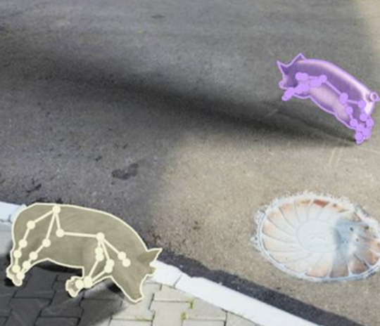
Our Research Lab at St. Petersburg mostly prefers PyTorch. For instance, we have used it for computer vision models that we applied to price tag segmentation. Here is a sample result:
But sometimes, especially in cases when PyTorch does not have a ready solution for something yet, we create our models in TensorFlow. The main idea of Neuromation idea is to train neural networks on synthetic data. We are convinced that a great result on real data can be obtained with transfer learning from perfectly labeled synthetic datasets. Have a look at some of our results for the segmentation of retail items based on synthetic data:
Conclusion
There are several deep learning frameworks, and we could go into a lot more detail about which to prefer. But, of course, frameworks are just tools to help you develop neural networks, and while the differences are important they are, of course, secondary. The primary tool in developing modern machine learning solutions is the neural network in your brain: the more you know, the more you think about machine learning solutions from different angles, the better you get. Knowing several deep learning frameworks can also help broaden your horizons, especially when the top contenders are as different as Theano and PyTorch. So it pays to learn them all even if your primary tool has already been chosen for you (e.g., your team uses a specific library). Good luck with your networks!
Oktai Tatanov Junior Researcher, Neuromation
Sergey Nikolenko Chief Research Officer, Neuromation
Our sixth installment of the NeuroNuggets series is slightly different from previous ones. Today we touch upon an essential and, at the same time, rapidly developing area — deep learning frameworks, software libraries that modern AI researchers and practitioners use to train all these models that we have been discussing in our first five installments. In today’s post, we will discuss what a deep learning framework should be able to do and see the most important algorithm that all of them must implement.
We have quite a few very talented junior researchers in our team. Presenting this post on neural networks’ master algorithm is Oktai Tatanov, our junior researcher in St. Petersburg:
What a Deep Learning Framework Must Do
A good AI model begins with an objective function. We also begin this essay with explaining the main purpose of deep learning frameworks. What does it mean to define a model (say, a large-scale convolutional network like the ones we discussed earlier), and what should a software library actually do to convert this definition into code that trains and/or applies the model?
Actually, every modern deep learning framework should be able to do the following checklist:
build and operate with large computational graphs;
perform inference (forward propagation) and automatic differentiation (backpropagation) on computational graphs;
be able to place the computational graph and perform the above operations on a GPU;
provide a suite of standard neural network layers and other widely used primitives that the computational graph might consist of.
As you can see, every point is somehow about computational graphs… but what are those? How does it relate to neural networks? Let us explain.
Computational Graphs: What
Artificial neural networks are called neural networks for a reason: they model, in a very abstract and imprecise way, processes that happen in our brains. In particular, neural networks consist of a lot of artificial neurons (perceptrons, units); outputs of some of the neurons serve as inputs for others, and outputs of the last neurons are the outputs of the network as a whole. Mathematically speaking, a neural network is a very large and complicated composition of very simple functions.
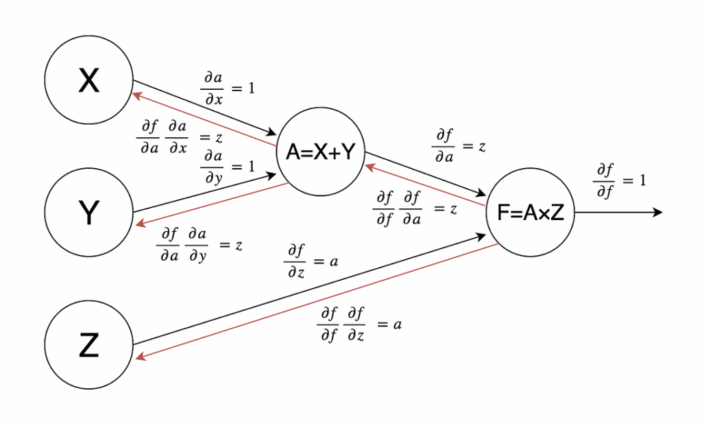
Computational graphs reflect the structure of this composition. A computational graph is a directed graph where every node represents a mathematical operation or a variable, and edges connect these operations with their inputs. As usual with graphs, a picture is worth a thousand words — here is a computational graph for the function :
The whole idea of neural networks is based on connectionism: huge compositions of very simple functions can give rise to very complicated behaviour. This has been proven mathematically many times, and modern deep learning techniques show how to actually implement these ideas in practice.
But why are the graphs themselves useful? What problem are we trying to solve with them, and what exactly are deep learning frameworks supposed to do?
Computational Graphs: Why
The main goal of deep learning is to train a neural network in such a way that it best describes the data we have. Most often, this problem is reduced to the problem of minimizing some kind of loss function or maximizing the likelihood or posterior distribution of a model, i.e., we either want to minimize how much our model gets wrong or want to maximize how much it gets right. The frameworks are supposed to help with these optimization problems.
Modern neural networks are very complicated and non-convex, so basically the only optimization method we have for large neural networks is the simplest and most universal optimization approach: gradient descent. In gradient descent, we basically compute the derivatives of the objective function (the gradient is the vector consisting of all partial derivatives) and then go into the direction where the objective function increases or decreases, as needed. Like this:
There are, of course, many interesting improvements and modifications to this simple idea: Nesterov’s momentum, adaptive gradient descent algorithms that change the learning rate separately for every weight… Perhaps one day we will return to this discussion in NeuroNuggets. But how do we compute the gradient if we have the neural network as model? That’s where computational graphs help…
Computational Graphs: How
To compute the gradient, deep learning frameworks use an algorithm called backpropagation (bprop); it basically amounts to using the chain rule sequentially across the computational graph. Let us walk through an application of backpropagation to our previous example. We begin by computing partial derivatives of every node of the graph with respect to each of its inputs; we assume that it is easy to do, and neural networks do indeed consist of simple units for which it is easy. Like in our example:
Now we need to combine these derivatives with the chain rule. In backpropagation, we do it sequentially from the graph’s output, where the objective function is computed. There we always have
Next, for example, we can get
since we already know both factors in this formula. Backpropagation means that we go through the graph from right to left, computing partial derivatives of f with respect to every node, including the weights that we are interested in. Here is the final result for our example:
This very simple algorithm allows us to set up algorithms to train any deep neural network. This is exactly what any deep learning framework is supposed to do; they are in reality automatic differentiation libraries more than anything else. The main function of any framework is to compute and take derivatives of huge compositions of functions. Note, by the way, that to compute the function you also need to traverse the computational graph, but this time from left to right, from variables to the outputs; this process is called forward propagation (fprop).
Parallelizing the Computations
Once you have the basic functionality of fprop and bprop in your library, you want to make it as efficient as possible. Efficiency gains mostly come from parallelization: note that operations in one part of the graph are completely independent from what happens in other parts. This means, for instance, that if you have a layer in your neural network, i.e., a set of nodes that do not feed into each other but all receive inputs from previous layers, you can compute them all in parallel during both forward propagation and backpropagation.
This is exactly the insight that to a large extent fueled the deep learning revolution: this kind of parallelization can be done across hundreds or even thousands of computational cores. What kind of hardware has thousands of cores? Why, the GPUs, of course! In 2009–2010, it turned out that regular off-the-shelf GPUs designed for gamers can provide a 10x-50x speedup in training neural networks. This was the final push for many deep learning models and applications into the territory of what is actually computationally feasible. We will stop here for the moment but hopefully will discuss parallelization in deep learning in much greater detail at some future post.
There is one more interesting complication. Deep learning frameworks come with two different forms of computational graphs, static and dynamic. Let us find out what this means.
Static and Dynamic Computational Graphs
The main idea of a static computational graph is to separate the process of building the graph and executing backpropagation and forward propagation (i.e., computing the function). Your graph is immutable, i.e., you can’t add or remove nodes at runtime.
In a dynamic graph, though, you can change the structure of the graph at runtime: you can add or remove nodes, dynamically changing its structure.
Both approaches have their advantages and disadvantages. For static graphs:
you can build a graph once and reuse it again and again;
the framework can optimize the graph before it is executed;
once a computational graph is built, it can be serialized and executed without the code that built the graph.
For dynamic graphs:
each forward pass basically defines a new graph;
debugging is easier;
constructing conditionals and loops is easy, which makes building recurrent neural networks much easier than with static graphs.
We will see live examples of code that makes use of dynamic computational graphs in the next installment, where we will consider several deep learning frameworks in detail. And now let us finish with an overview.
Deep Learning Frameworks: An Overview
On March 10, Andrej Karpathy (Director of AI at Tesla) published a tweet with very interesting statistics about machine learning trends. Here is the graph of unique mentions of deep learning frameworks over the last four years:
The graph shows that the top 4 general-purpose deep learning frameworks right now are TensorFlow, Caffe, Keras, and PyTorch, while, for example, historically the first widely used framework theano has basically lost traction.
The frameworks have interesting relations between them, and it is worthwhile to consider them all, get a feeling of what the code looks like for each, and discuss their pros and cons. This post, however, is already growing long; we will come back to this discussion in the second part.
Oktai Tatanov Junior Researcher, Neuromation
Sergey Nikolenko Chief Research Officer, Neuromation
This week, we continue the NeuroNuggets series with the fifth installment on another important computer vision problem: pose estimation. We have already talked about segmentation; applied to humans, segmentation would mean to draw silhouettes around pictures of people. But what about the skeleton? We need pose estimation, in particular, to understand what a person is doing: running, standing, reading NeuroNuggets?
Today, we present a pose estimation model based on the so-called Part Affinity Fields (PAF), a model from this paper that we have uploaded on the NeuroPlatform as a demo. And presenting this model today is Arseny Poezzhaev, our data scientist and computer vision aficionado who has moved from Kazan to St. Petersburg to join Neuromation! We are excited to see Arseny join and welcome him to the team (actually, he joined from the start, more than a month ago, but the NeuroNuggets duty caught up only now). Welcome:
Introduction
Pose estimation is one of the long-standing problems of computer vision. It has interested researchers over the last several decades because not only is pose estimation an important class of problems itself, but it also serves as a preprocessing step for many even more interesting problems. If we know the pose of a human, we can further train machine learning models to automatically infer relative positions of the limbs and generate a pose model that can be used to perform smart surveillance with abnormal behaviour detection, analyze pathologies in medical practices, control 3D model motion in realistic animations, and a lot more.
Moreover, not only humans can have limbs or a pose! Basically, pose estimation can deal with any composition of rigidly moving parts connected to each other at certain joints, and the problem is to recover a representative layout of body parts from image features. We at Neuromation, for example, have been doing pose estimation for synthetic images of pigs (cf. our Piglet’s Big Brother project):
Traditionally, pose estimation used to be done by retrieving motion patterns from optical markers attached to the limbs. Naturally, pose estimation would work much better if we could afford to put special markers on every human on the picture; alas, our problem is a bit harder. The next point of distinction between different approaches is the hardware one can use: can we use multiple cameras? 3D cameras that estimate depth? infrared? Kinect? is there a video stream available or only still images? Again, each additional source of data can only make the problem easier, but in this post we concentrate on a single standard monocular camera. Basically, we want to be able recognize the poses on any old photo.
Top-Down and Bottom-Up
Pose estimation from a single image is a very under-constrained problem precisely due to the lack of hints from other channels, different viewpoints from multiple cameras, or motion patterns from video. The same pose can produce quite different appearances from different viewpoints and, even worse, human body has many degrees of freedom, which means that the solution space has high dimension (always a bad thing, trust me). Occlusions are another big problem: partially occluded limbs cannot be reliably recognized, and it’s hard to teach a model to realize that a hand is simply nowhere to be seen. Nevertheless, single person pose estimation methods show quite good results nowadays.
When you move from a single person to multiple people, pose estimation becomes even harder: humans occlude and interact with other humans. In this case, it is common practice to use a so-called top-down approach: apply a separately trained human detector (based on object detection techniques such as the ones we discussed before), find each person, and then run pose estimation on every detection. It sounds reasonable but actually the difficulties are almost insurmountable: if the detector fails to detect a person, or if limbs from several people appear in a single bounding box (which is almost guaranteed to happen in case of close interactions or crowded scenes), the whole algorithm will fail. Moreover, the computation time needed for this approach grows linearly with the number of people on the image, and that can be a big problem for real-time analysis of groups of people.
In contrast, bottom-up approaches recognize human poses from pixel-level image evidence directly. They can solve both problems above: when you have information from the entire picture you can distinguish between the people, and you can also decouple the runtime from the number of people on the frame… at least theoretically. However, you are still supposed to be able to analyze a crowded scene with lots of people, assigning body parts to different people, and even this task by itself could be NP-hard in the worst case.
Still, it can work; let us show which pose estimation model we chose for the Neuromation platform.
It is a bottom-up approach, and it uses the so-called Part Affinity Fields (PAFs) together with estimation of body-part confidence maps. PAFs are the main new idea we introduce today, so let us discuss them in a bit more detail. A PAF is a set of 2D vector fields that encode the location and orientation of the limbs. Vector fields? Sounds mathy… but wait, it’s not that bad.
Suppose you have already detected all body parts (hands, elbows, feet, ankles etc.); how do you now generate poses from them? First, you must find out how to connect two points to form a limb. For each body part, there are several candidates to form a limb: there are multiple people on the image, and there also can be lots of false positives. We need some confidence measure for the association between each body part detection. Cao et al. propose a novel feature representation called Part Affinity Fields that contains information about location as well as orientation across the region of support of the limb.
In essence a PAF is a set of vectors that encodes the direction from one part of the limb to the other; each limb is considered as an affinity field between body parts. Here is a forehand:
Figure 1. Affinity field visualization for right forehand. The color encodes limb’s orientation.
If a point lies on the limb then its value in the PAF is a unit vector pointing from starting joint point to ending joint point of this limb; the value is zero if it is outside the limb. Thus, PAF is a vector field that contains information about one specific limb for all the people on the image, and the entire set of PAFs encodes all the limbs for every person. So how do PAFs help us for pose estimation?
Method overview
First, let us go through the overall pipeline of the algorithm.
Figure 2 above illustrates all the steps from an input image (Fig. 2a) to anatomical keypoints as an output (Fig. 2e). First, a feedforward neural network predicts a set of body part locations on the image (Fig. 2b) in the form of a confidence map and a set of PAFs that encode the degree of association between these body parts (Fig. 2c). Thus, the algorithm gets all information necessary for further matching of limbs and people (all of this stuff does sound a bit bloodthirsty, doesn’t it?). Next, confidence maps and affinity fields are parsed together (Fig 1d) to output the final positions of limbs for all people on the picture.
All of this sounds very reasonable: we now have a plan. But so far this is only a plan: we don’t know how to do any of these steps above. So now let us consider every step in detail.
Architecture
One of the core ideas of (Cao et al., 2017) is to simultaneously predict detection confidence map and affinity fields. The method uses a special feedforward network as a feature extractor. The network looks like this:
Figure 3. Architecture of the two-branch multistage CNN. Each stage in the top branch (beige) predicts a confidence map S, and each stage in the bottom branch (blue) predicts a PAF L. After every stage, predictions from both branches are concatenated with image features F (which come from a VGG-based architecture) and used as input for the next stage. Each branch performs multiple inferences, one per body part.
As you can see, it is split into two branches: the top branch predicts the detection confidence maps and the bottom branch is for affinity fields. Both branches are organized as an iterative prediction architecture, which refines predictions over successive stages. The improvement of accuracy of predictions is controlled by intermediate supervision at each stage. Here is how it might look on a real image:
Figure 4. Demonstration of real image inference by the two-branched architecture neural network.
Before passing input to this two-branch network the method uses auxiliary CNN (first 10 layers of VGG-19) to extract an input feature map F. This prediction is processed by both branches, and their predictions concatenated with initial F are used as input for the next stage (as features).
This process is repeated on every stage, and you can see the refinement process across stages on Figure 4 above.
From Body Parts to Limbs
Take a look at Figure 5 below, which again illustrates the above-mentioned refinement process:
Figure 5. Confidence maps of right wrist (first row) and PAFs of right forearm (second row) across stages. We can see that despite confusion on the first stage, the method can fix its mistakes on later stages.
At the end of each stage, the corresponding loss function is applied for each branch to guide the network.
Now consider the top branch; each confidence map is a 2D representation of our confidence that each pixel belongs to a particular body part (we remind that “body parts” here are “points” such as wrists and elbows, and, say, forearms are referred to as “limbs” rather than “body parts”). To get body part candidate regions, we aggregate confidence maps for different people. After that, the algorithm performs non-maximum suppression to obtain a discrete set of parts locations:
Figure 6. How algorithm forms limbs from detections.
During inference, algorithm computes line integrals over all the PAFs along the line segments between pairs of detected body-parts. If the candidate limb formed by connection of certain pair of points is aligned with corresponding PAF then it’s considered as a true limb. This is exactly what the bottom branch does.
From Limbs to Full Body Models
We now see how the algorithm can find limbs on the image between two points. But we still cannot estimate poses because we need the full body model! We need to somehow connect all these limbs into people. Formally speaking, the algorithm has found body part candidates and has scored pairs of these parts (integrating over PAFs), but the final goal is to find the optimal assignment for the set of all possible connections.
Formally speaking, this problem can be viewed as a k-partite graph matching problem, where nodes of the graph are body part detections, and edges are all possible connections between them (possible limbs). Here k-partite matching means that the vertices can be partitioned into k groups of nodes with no connections inside each group (i.e., vertices corresponding to the same body part). Edges of the graph are weighted with part affinities. Like this:
A direct solution of this problem may be computationally infeasible (NP-hard), so (Cao et al., 2017) propose a relaxation where the initial k-partite graph is decomposed into a set of bipartite graphs (Fig. 7d) where the matching task is much easier to solve. The decomposition is based on the problem domain: basically, you know how body parts can connect, and a hip cannot be connected to a foot directly, therefore we can first connect hip to knee and then knee to foot.
That’s all, folks! We have considered all the steps in the algorithm that can retrieve poses from a single raw image. Let us now see how it works on our platform.
Pose Estimation Demo in Action
There are, as always, a few simple steps to run this algorithm on our image of interest:
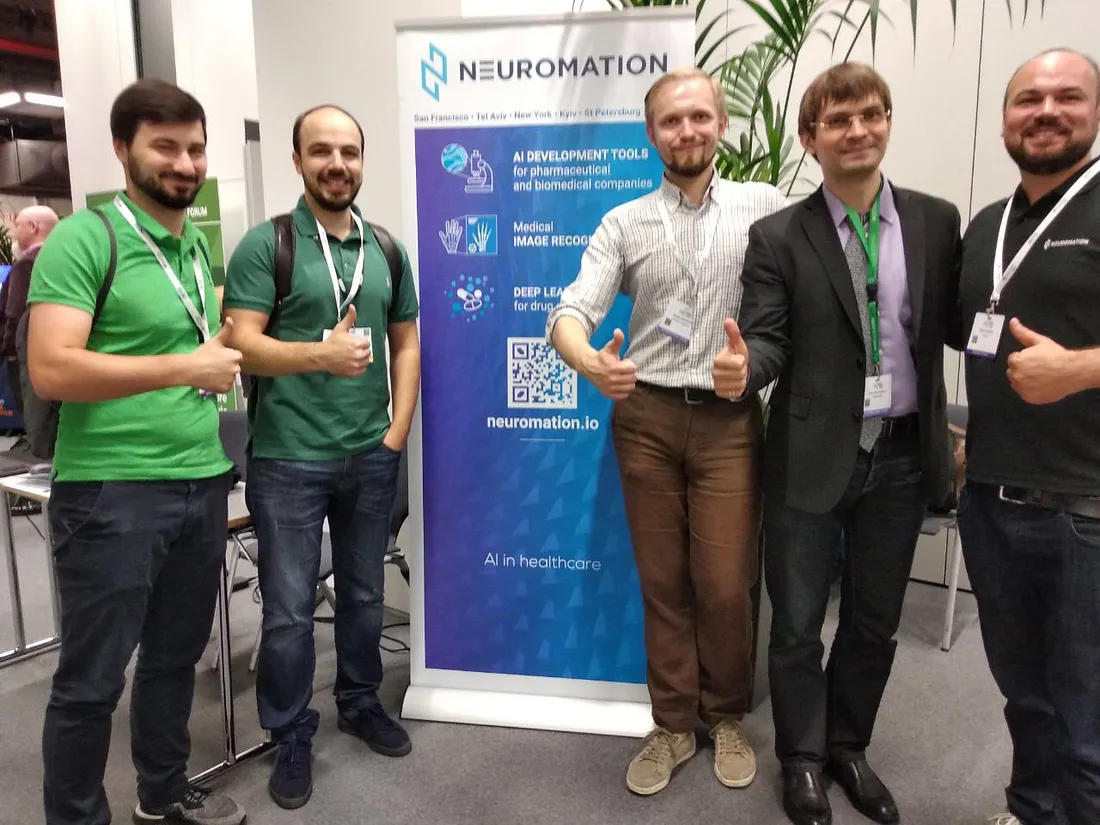
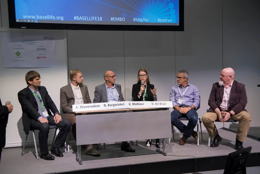
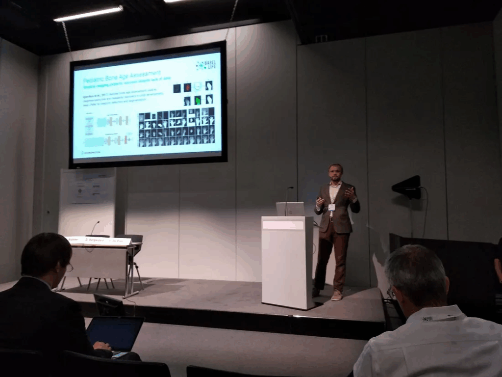


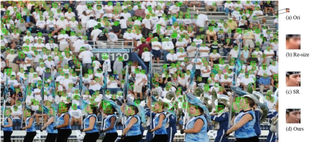
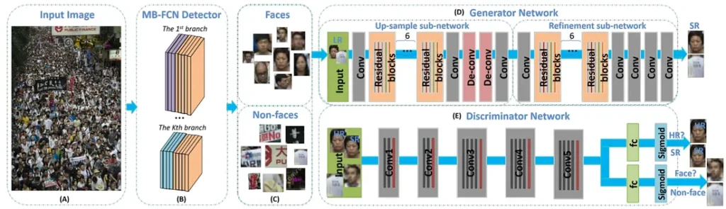
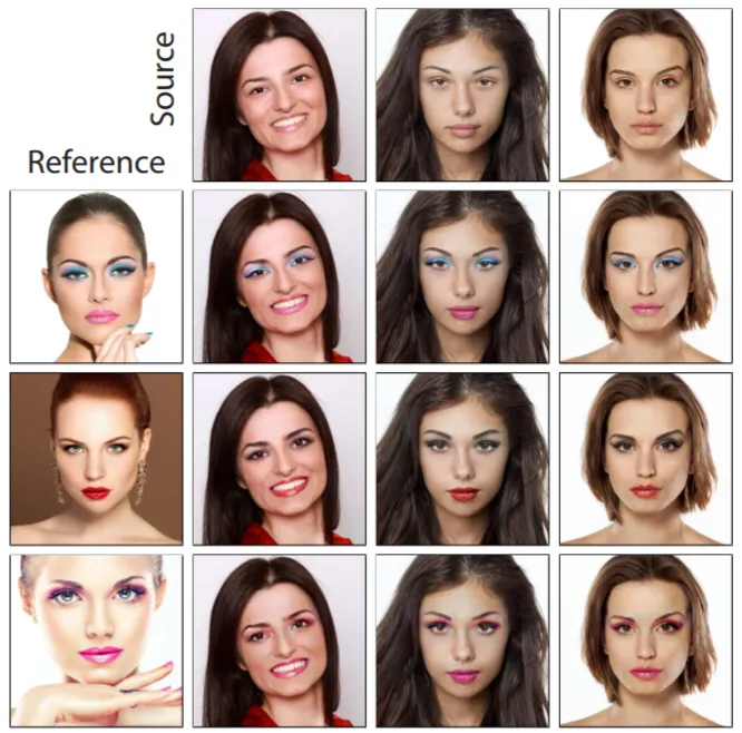
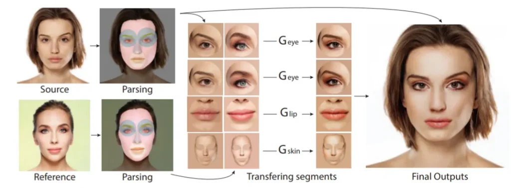
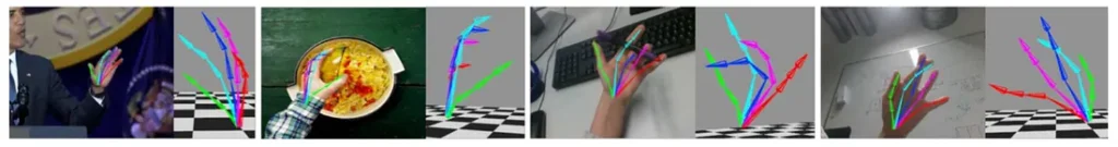
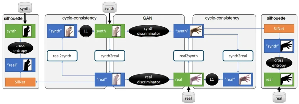
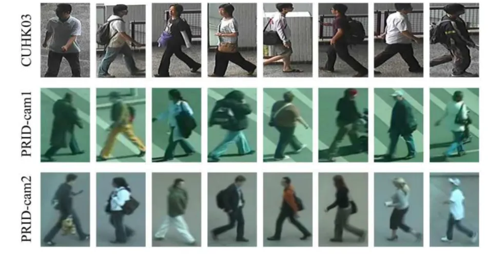
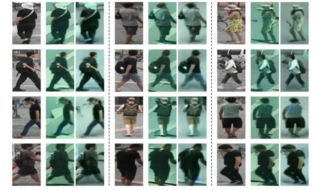
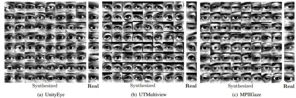
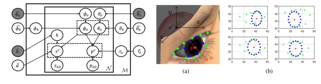
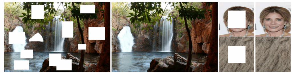
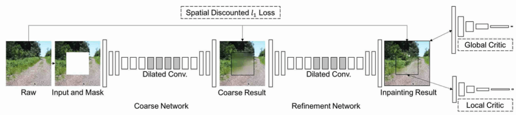
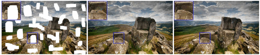
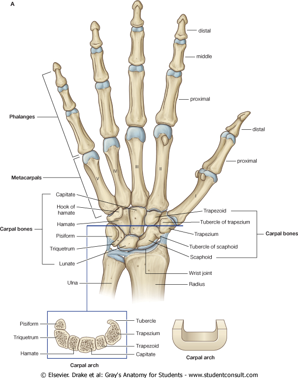
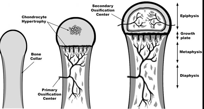
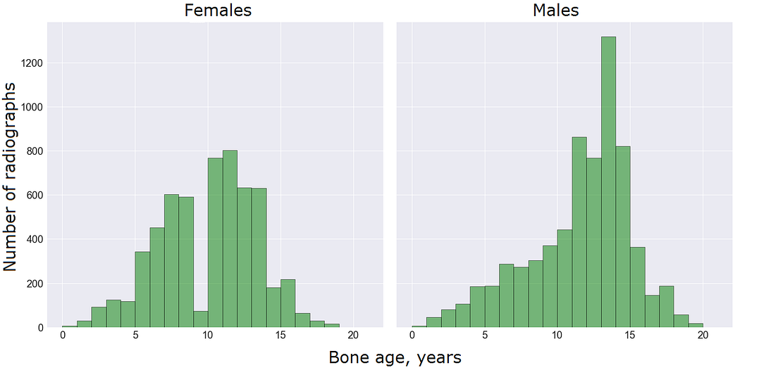
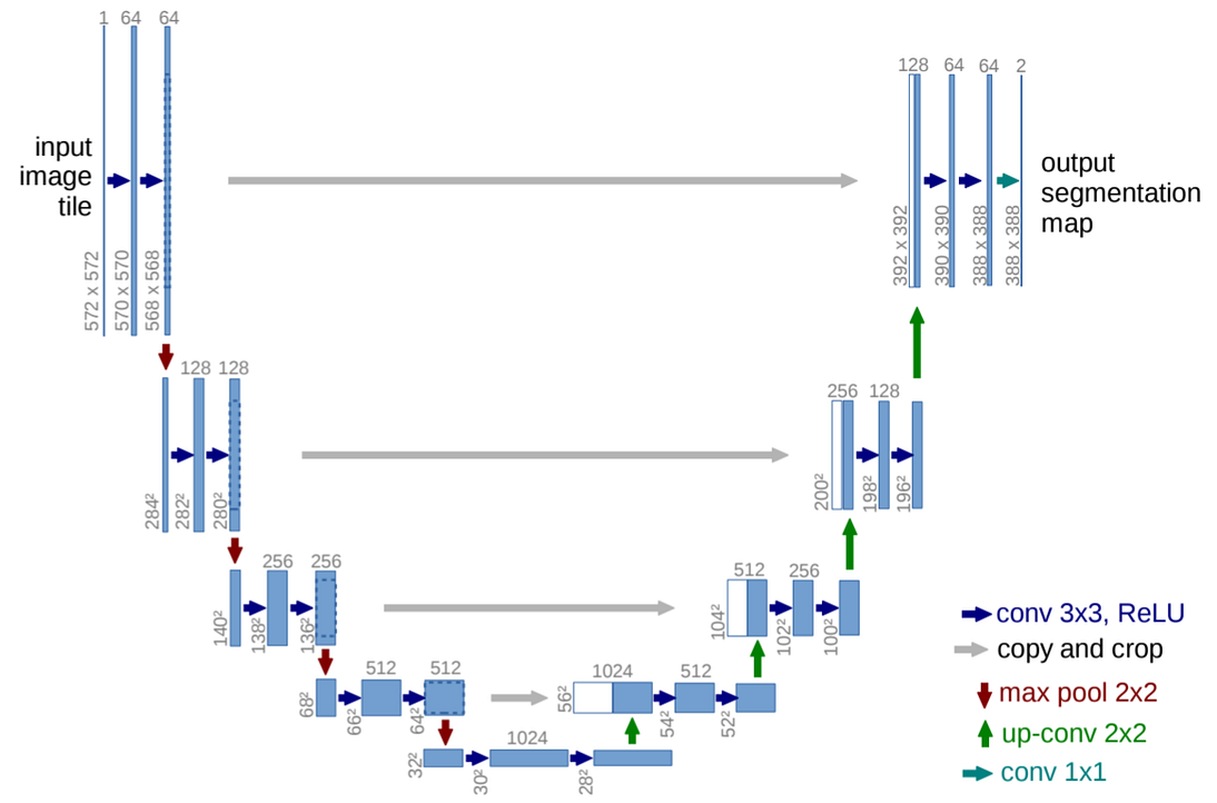
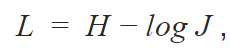
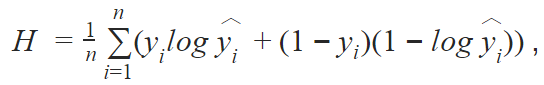


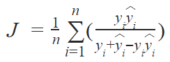
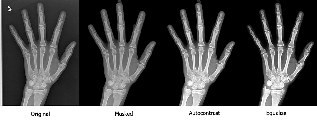
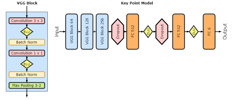
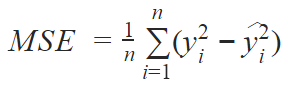
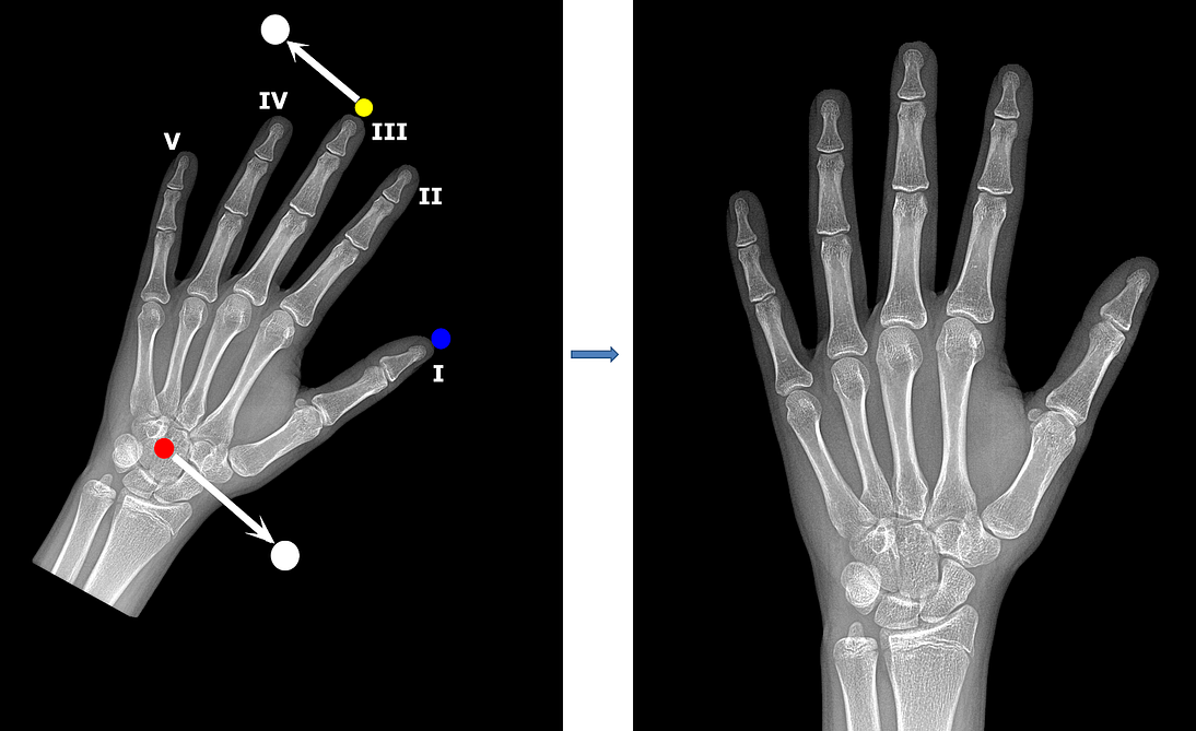
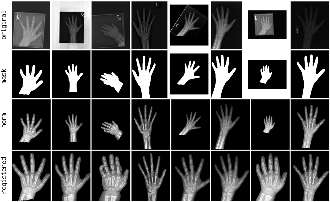
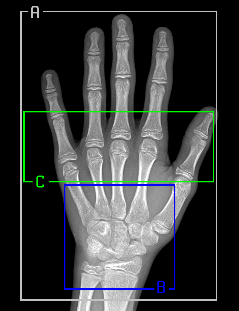
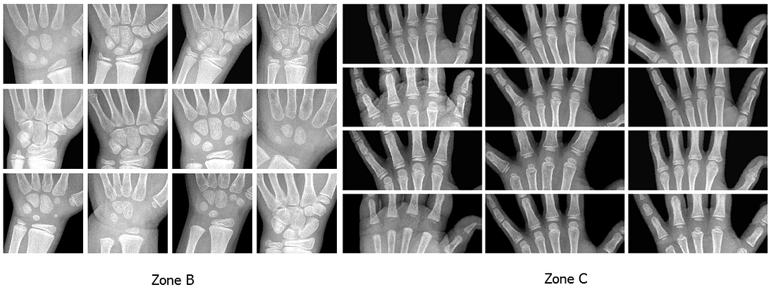
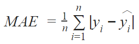
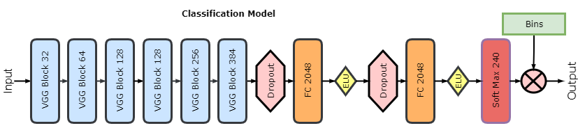
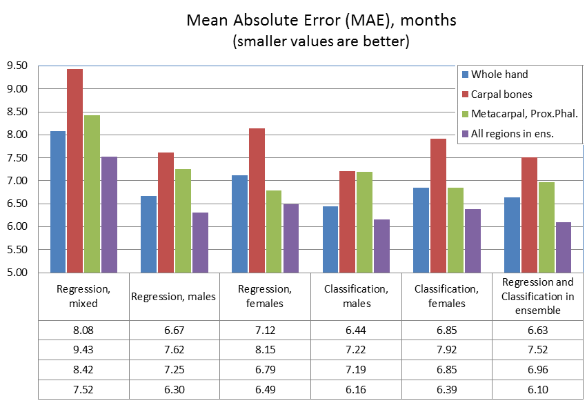

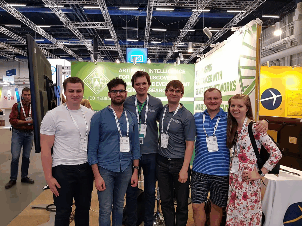
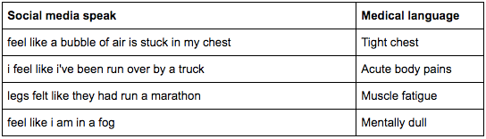
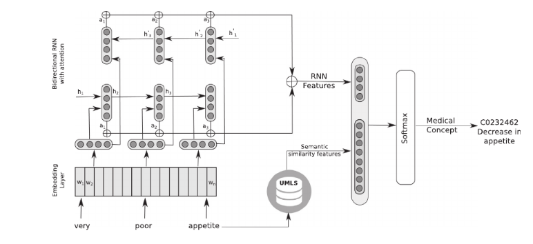
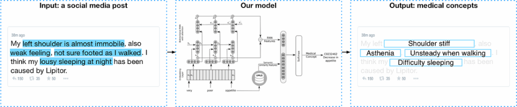
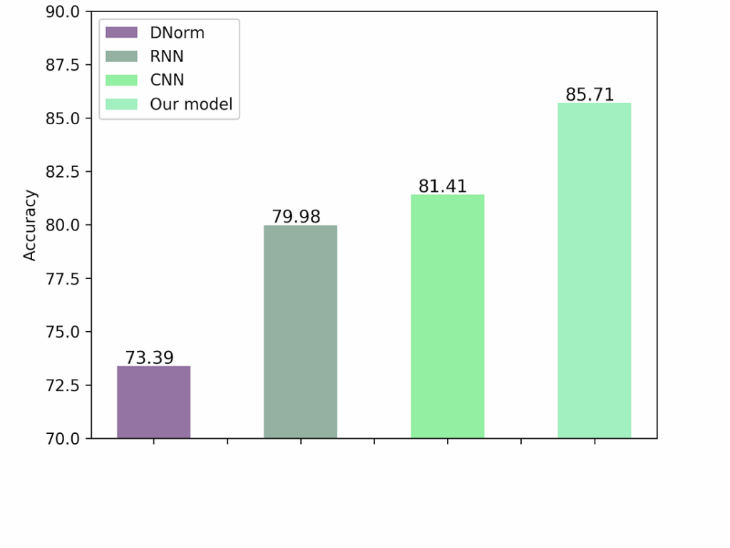


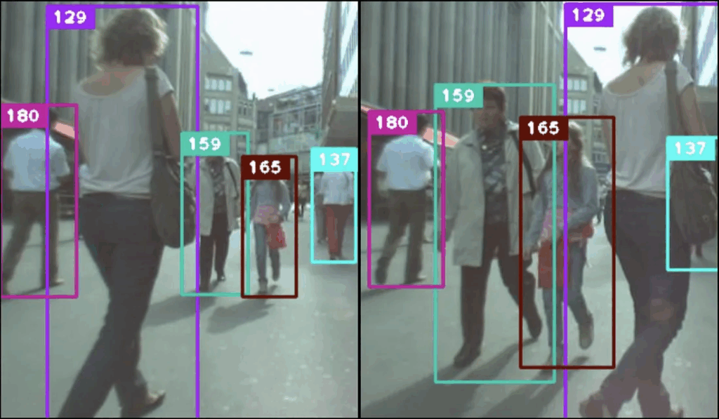
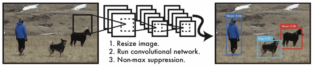
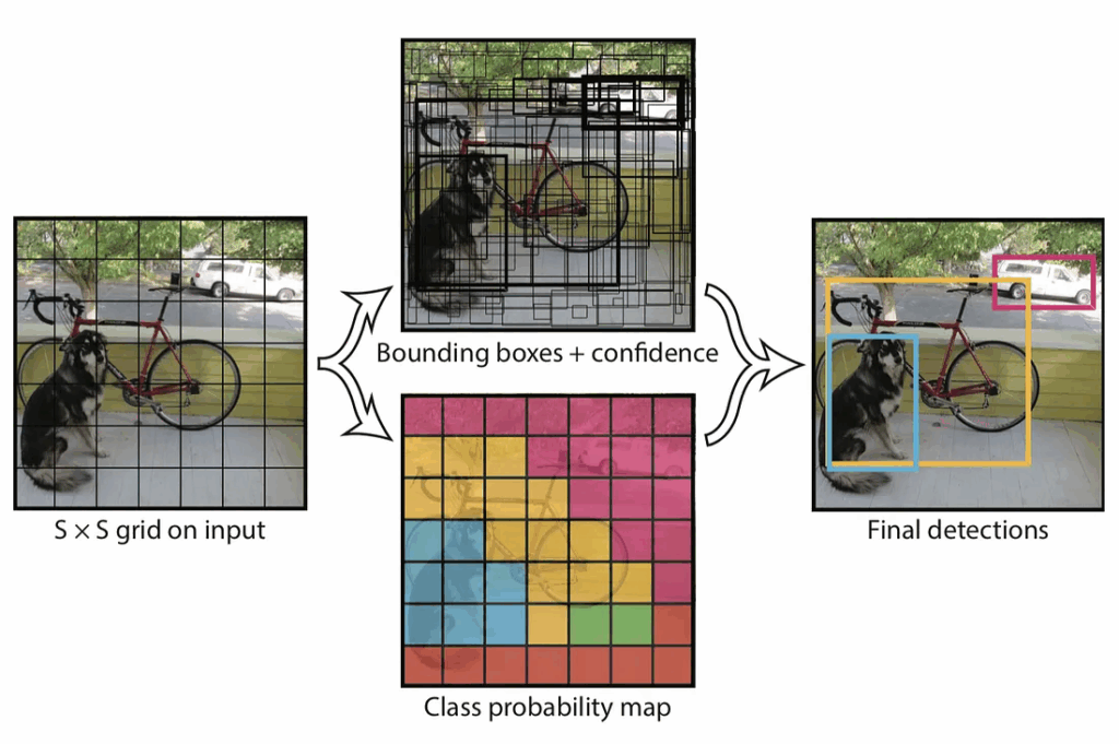
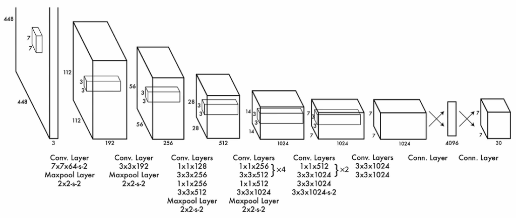
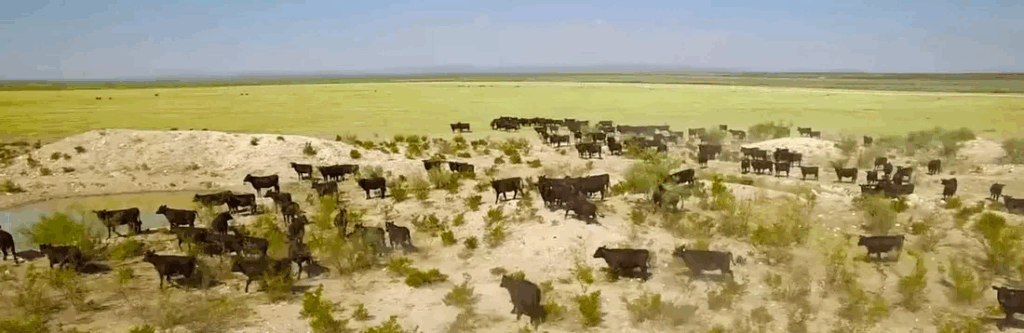
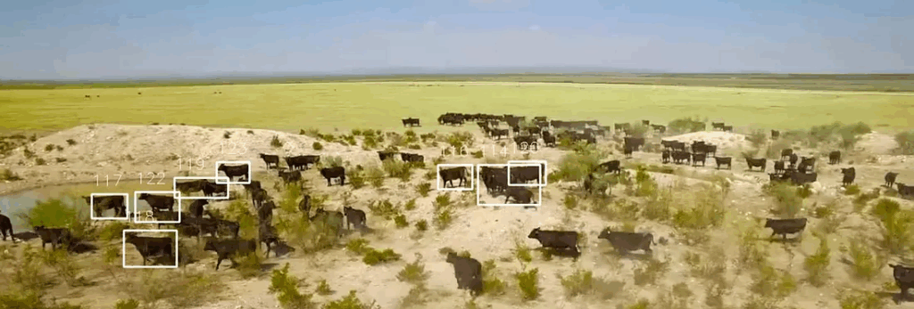
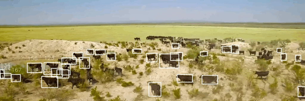
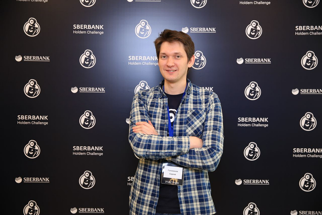

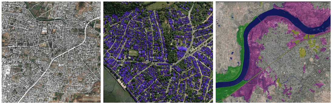
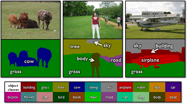
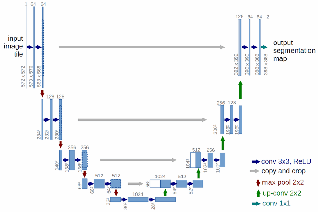
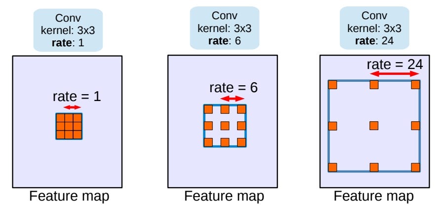
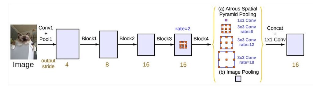
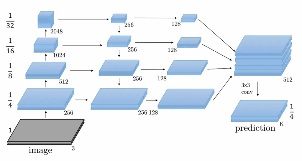
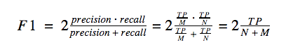
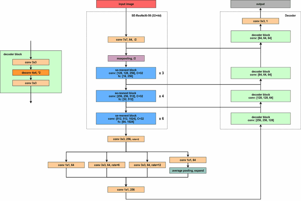
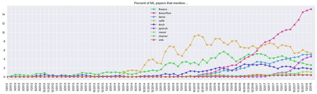
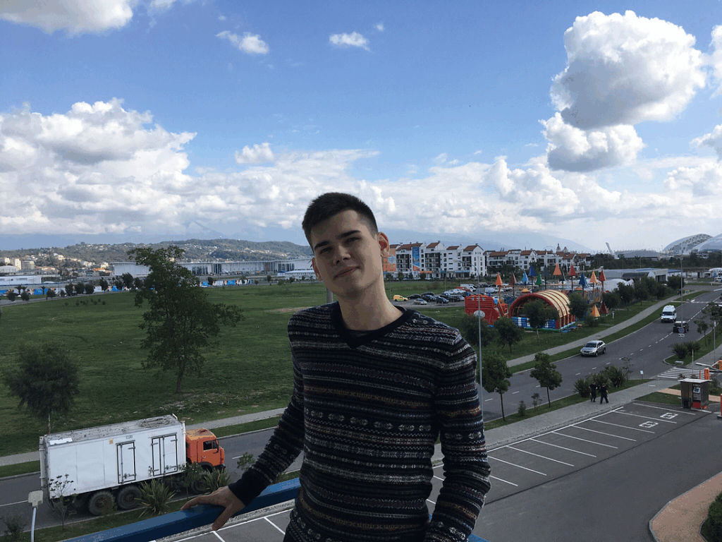
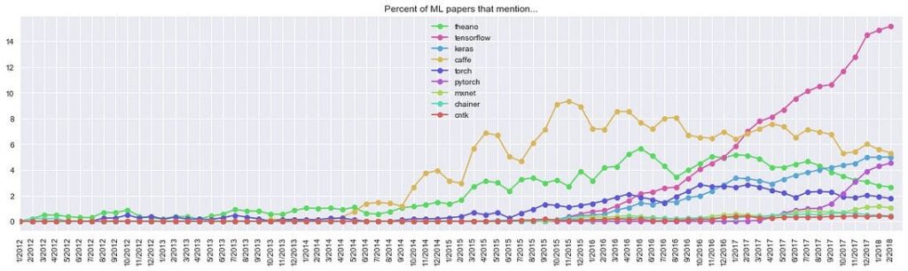
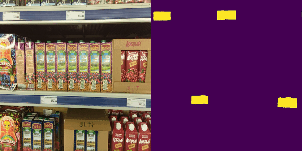
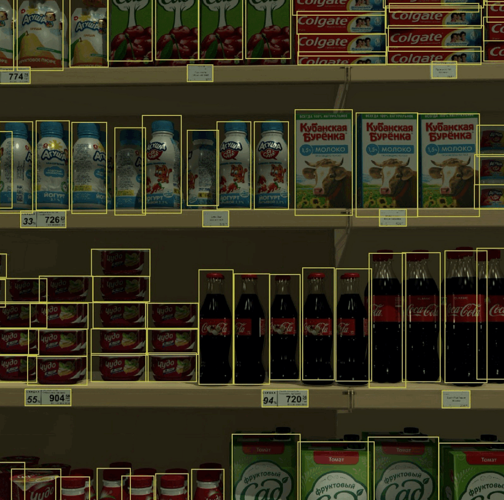
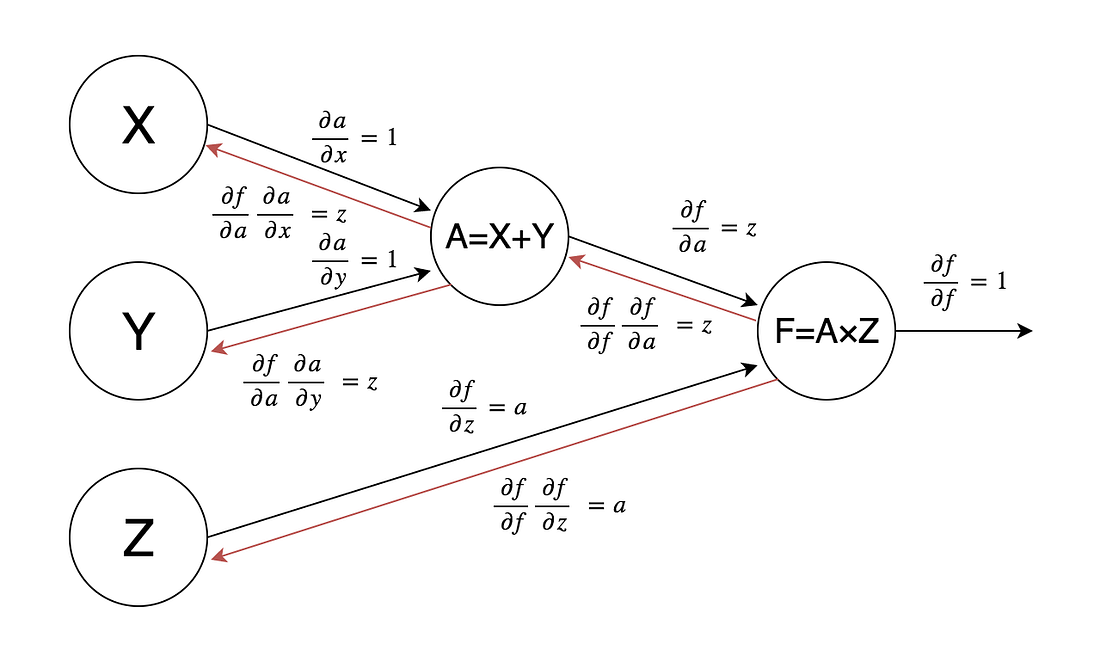
 :
: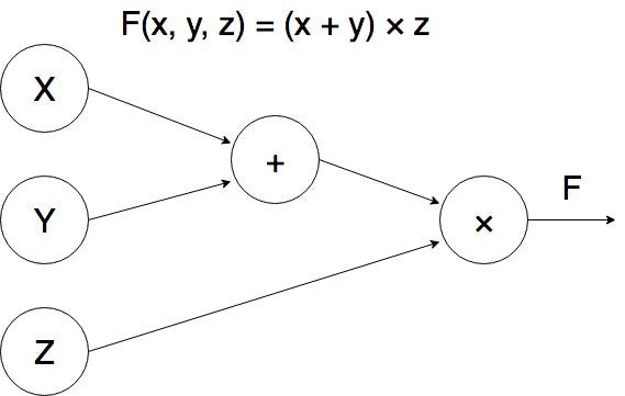
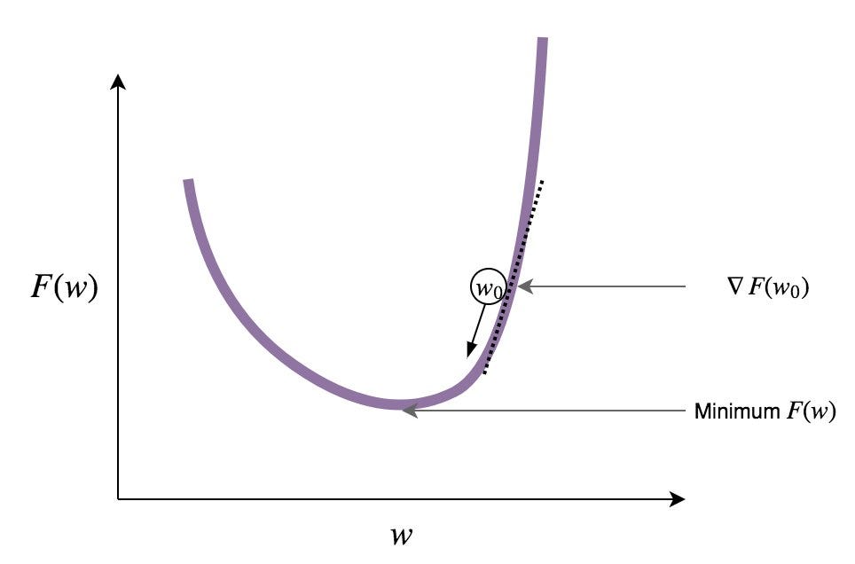
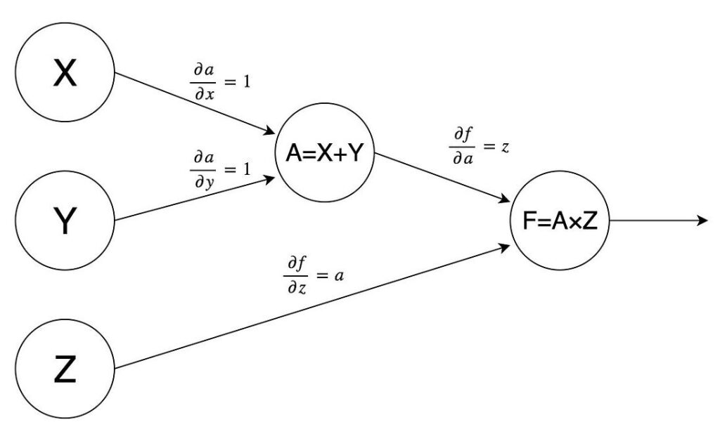
![\[\frac{\partial f}{\partial f} = 1.\]](https://blog.sergeynikolenko.ru/wp-content/ql-cache/quicklatex.com-fd57f85c15062124d620ce58deaa431e_l3.svg "Rendered by QuickLaTeX.com")
![\[\frac{\partial f}{\partial x} = \frac{\partial f}{\partial a}\frac{\partial a}{\partial x}= z\cdot 1 = z,\]](https://blog.sergeynikolenko.ru/wp-content/ql-cache/quicklatex.com-60b06c10594b646385152c2fb7bb610d_l3.svg "Rendered by QuickLaTeX.com")