А это просто хороший survival horror в стиле игр с PlayStation 1. После того как мне (немного неожиданно для самого себя) зашёл Signalis, я решил попробовать другого представителя жанра. И не был разочарован!
Здесь нет никакой суперзагадочной истории: ты детектив, приезжающий в заброшенный парк развлечений искать пропавших людей и хозяина парка. Дальше, конечно, происходит много странного и антинаучного, нападают странные мутанты, но история разворачивается достаточно логично, записки объясняют весь контекст, и следить за происходящим интересно. Есть только один небольшой твист в конце, который ни на что не влияет (и на самом деле непонятно зачем добавлен).
Собственно, и хоррора никакого нет: не было даже того постоянного дискомфорта и давящей атмосферы, которые создаёт Signalis. А в Crow Country вся рисовка скорее мультяшная, скримеров никаких нету, и даже чересчур неприятных вещей ни с кем не происходит.
Но мне очень понравились загадки; они не совсем тривиальные, но достаточно простые. Так что получается, что ты нигде не застреваешь (та редкая игра, где я ни разу не пользовался гайдами), а просто идёшь вперёд и решаешь загадку за загадкой… но тебе при этом не скучно! В Crow Country есть даже карта секретов, которая сразу показывает, в каких комнатах их искать. В итоге я после обычного прохождения получил все achievements, кроме одного, которое требует перепрохождения — да, там есть что-то вроде NG+, но туда я уже не полез, конечно.
В общем, рекомендую любителям жанра, да и нелюбителей эта игра может переубедить.
Сергей Николенко
P.S. Прокомментировать и обсудить пост можно в канале “Sineкура”: присоединяйтесь!
Это. Просто. Хорошая. Метроидвания. Абсолютно стандартная, по канонам. Рисованные мышки спасают свой маленький мир от злых роботов и прочих созданий. Мыш, за которого мы играем, получает новые способности вроде двойного прыжка или приклеивания к стенкам, что открывает новые проходы в разных местах. После победы над боссом летающие острова приклеиваются друг к другу, что тоже открывает новые проходы.
Но хорошо сделано! Прыгать приятно, сражаться приятно, летать на небольшом деревянном самолётике приятно, арт-стиль милый, боссы нетривиальные, но не душные, история ни на что не претендующая, но с забавными шуточками. Вот просто всё сделано компетентно и с любовью, нет ни одной провальной стороны.
И в результате игра, которая снаружи кажется стандартной, чуть ли не унылой и не имеющей никакой особой фишки, на самом деле восхитительно играется. С большим удовольствием прошёл и всем рекомендую; это для меня примерно такой же hidden gem, каким когда-то оказался Teslagrad в жанре пазл-платформеров. Надо будет, кстати, рассказать про него при случае.
Сергей Николенко
P.S. Прокомментировать и обсудить пост можно в канале “Sineкура”: присоединяйтесь!
Современные LLM, даже рассуждающие, всё равно очень плохи в алгоритмических задачах. И вот, кажется, намечается прогресс: Hierarchical Reasoning Model (HRM), в которой друг с другом взаимодействуют две рекуррентные сети на двух уровнях, с жалкими 27 миллионами параметров обошла системы в тысячи раз больше на задачах, требующих глубокого логического мышления. Как у неё это получилось, и может ли это совершить новую мини-революцию в AI? Давайте разберёмся…
Судоку, LLM и теория сложности
Возможности современных LLM слегка парадоксальны: модели, которые пишут симфонии и объясняют квантовую хромодинамику, не могут решить судоку уровня «эксперт». На подобного рода алгоритмических головоломках точность даже лучших LLM в мире стремится к нулю.
Это не баг, а фундаментальное ограничение архитектуры. Вспомните базовый курс алгоритмов (или менее базовый курс теории сложности, если у вас такой был): есть задачи класса P (решаемые за полиномиальное время), а есть задачи, решаемые схемами постоянной глубины (AC⁰). Трансформеры, при всей их мощи, застряли во втором классе, ведь у них фиксированная и не слишком большая глубина.
Представьте это так: вам дают лабиринт и просят найти выход. Это несложно, но есть нюанс: смотреть на лабиринт можно ровно три секунды, вне зависимости от того, это лабиринт 5×5 или 500×500. Именно так работают современные LLM — у них фиксированное число слоёв (обычно несколько десятков), через которые проходит информация. Миллиарды и триллионы параметров относятся к ширине обработки (числу весов в каждом слое), а не к глубине мышления (числу слоёв).
Да, начиная с семейства OpenAI o1 у нас есть “рассуждающие” модели, которые могут думать долго. Но это ведь на самом деле “костыль”: они порождают промежуточные токены, эмулируя цикл через текст. Честно говоря, подозреваю, что для самой LLM это как программировать на Brainfuck — технически возможно, но мучительно неэффективно. Представьте, например, что вам нужно решить судоку с такими ограничениями:
смотреть на картинку можно две секунды,
потом нужно записать обычными словами на русском языке то, что вы хотите запомнить,
и потом вы уходите и возвращаетесь через пару дней (полностью “очистив контекст”), получая только свои предыдущие записи на естественном языке плюс ещё две секунды на анализ самой задачи.
Примерно так современные LLM должны решать алгоритмические задачи — так что кажется неудивительным, что они это очень плохо делают!
И вот Wang et al. (2025) предлагают архитектуру Hierarchical Reasoning Model (HRM), которая, кажется, умеет думать нужное время естественным образом:
Как работает HRM? Как бы избито и устарело это ни звучало, будем опять вдохновляться нейробиологией…
Тактовые частоты мозга и архитектура HRM
Нейробиологи давно знают, что разные области коры головного мозга работают на разных “тактовых частотах”. Зрительная кора обрабатывает информацию за миллисекунды, префронтальная кора “думает” секундами, а гиппокамп может удерживать паттерны минутами (Murray et al., 2014; Zeraati et al., 2023). Эти timescales измеряются обычно через временные автокорреляции между сигналами в мозге, результаты устойчивы для разных модальностей, и учёные давно изучают и откуда это берётся, и зачем это нужно (Zeraati et al., 2024):
Это не случайность, а элегантное решение проблемы вычислительной сложности. Быстрые модули решают локальные подзадачи, медленные — координируют общую стратегию. Как дирижёр оркестра не играет каждую ноту, но задаёт темп и структуру всему произведению, а конкретные ноты играют отдельные музыканты.
Авторы Hierarchical Reasoning Model (HRM) взяли эту идею и применили её к рекуррентным сетям. Глубокие рекуррентные сети, у которых второй слой получает на вход скрытые состояния или выходы первого и так далее, конечно, давно известны, но что если создать рекуррентную архитектуру с двумя взаимодействующими уровнями рекуррентности? Верхний уровень будет получать результат нескольких шагов нижнего уровня, возможно уже после сходимости, и работать медленнее:
Идея настолько простая, что даже удивительно, почему её не попробовали раньше (а может, уже пробовали?). По сути, мы просто обучаем две вложенные рекуррентные сети:
быстрый модуль (L) выполняет T шагов вычислений, сходясь к локальному решению;
медленный модуль (H) обновляется раз в T шагов, меняя тем самым контекст для быстрого модуля.
Но дьявол, как всегда, в деталях. Просто соединить две RNN-архитектуры недостаточно — они или быстро сойдутся к фиксированной точке и перестанут что-либо вычислять, или будут требовать огромных ресурсов для обучения. Нужны ещё трюки, и в HRM они довольно простые, так что давайте их тоже рассмотрим.
Важные трюки
Трюк №1: Иерархическая сходимость
Вместо одной большой задачи оптимизации HRM решает последовательность связанных задач. Быстрый модуль сходится, потом медленный модуль обновляется, и появляется новая точка сходимости для быстрого модуля. Для быстрого модуля всё выглядит как решение последовательности связанных, но всё-таки разных задач, и ему всё время есть куда двигаться. Это хорошо видно на графиках сходимости:
Трюк №2: Backpropagation, But Not Through Time
Обычно рекуррентные сети обучаются при помощи так называемого backpropagation through time (BPTT): нужно запомнить все промежуточные состояния, а потом распространить градиенты назад во времени. Хотя это вполне естественно для обучения нейросети, это требует много памяти и вычислительных ресурсов, а также, честно говоря, биологически неправдоподобно: мозг же не хранит полную историю всех активаций своих синапсов, у мозга есть только текущее состояние.
Получается, что хранить нужно только текущие состояния сетей; O(1) памяти вместо O(T)! Конечно, это не то чтобы сложная идея, и при обучении обычных RNN у неё есть очевидные недостатки, но в этом иерархическом случае, похоже, работает неплохо.
Трюк №3: Адаптивное мышление через Q-learning
Не все задачи одинаково сложны. HRM может “думать дольше” над трудными проблемами, используя механизм адаптивной остановки, обученный через reinforcement learning. Если судоку на 80% заполнено, то скорее всего хватит и пары итераций, а в начале пути придётся крутить шестерёнки иерархических сетей подольше. Это тоже не новая идея — Alex Graves ещё в 2016 предлагал adaptive computation time for RNNs — но в этом изводе результаты действительно впечатляющие, всё хорошо обучается и работает:
Результаты
Экспериментальные результаты тут, конечно, крайне впечатляющие. Можно сказать, переворачивают представление о том, что такое “эффективность” в AI.Всего с 27 миллионами параметров, обучаясь примерно на 1000 примеров, HRM получила:
40.3% на ARC-AGI-1 (тест на абстрактное мышление, где o3-mini даёт 34.5%, а Claude — 21.2%);
55% точных решений для экстремально сложных судоку (здесь рассуждающие модели выдают устойчивый ноль решений);
74.5% оптимальных путей в лабиринтах 30×30 (где, опять же, рассуждающие модели не делают ничего разумного).
Для контекста скажу, что задачи действительно сложные; например, судоку в тестовом наборе требуют в среднем 22 отката (backtracking) при решении алгоритмическими методами, так что это не головоломки для ленивого заполнения в электричке, а сложные примеры, созданные, чтобы тестировать алгоритмы. Вот, слева направо, примеры заданий из ARC-AGI, судоку и лабиринтов:
Заглядываем под капот: как оно думает?
В отличие от больших моделей, у которых интерпретируемость потихоньку развивается, но пока оставляет желать лучшего, HRM позволяет наглядно визуализировать процесс мышления:
Здесь хорошо видно, что:
в лабиринтах HRM сначала исследует множество путей параллельно, потом отсекает тупики;
в судоку получается классический поиск в глубину — заполняет клетки, находит противоречия, откатывается;
а в ARC-задачах всё это больше похоже на градиентный спуск в пространстве решений.
Спонтанная иерархия размерностей
Я начал этот пост с аналогии с мозгом. Они часто в нашей науке появляются, но обычно не имеют особенно глубокого смысла: в мозге нет backpropagation, как следствие там совсем другая структура графа вычислений, и аналогии редко выдерживают этот переход. Но в данном здесь параллель оказалась глубже, чем даже изначально предполагали авторы. После обучения в HRM сама собой развивается “иерархия размерностей” — высокоуровневый модуль работает в пространстве примерно в 3 раза большей размерности, чем низкоуровневый (центральный и правый столбцы):
И оказывается, то точно такая же организация наблюдается в мозге мыши (Posani et al., 2025; левый столбец на картинке выше)!
Этот эффект не был задан через гиперпараметры, а возник сам собой, эмерджентно из необходимости решать сложные задачи. Тут, конечно, результат не настолько мощный, чтобы рассуждать о каком-то фундаментальном принципе организации иерархических вычислений, который независимо открывают и биологическая эволюция, и градиентный спуск… но вот я уже порассуждал, и звучит довольно правдоподобно, честно говоря.
Заключение: ограничения и философствования
Во-первых, давайте всё-таки не забывать важные ограничения HRM:
все тесты были сделаны на структурированных задачах (судоку, лабиринты), а не на естественном языке;
результаты на ARC сильно зависят от test-time augmentation (1000 вариантов каждой задачи);
для идеального решения судоку нужны все 3.8M обучающих примеров, а не заявленные 1000.
И главный вопрос, на который пока нет ответа: масштабируется ли это до размеров современных LLM? Если да, то это может быть важный прорыв, но пока, конечно, ответа на этот вопрос мы не знаем.
И тем не менее, HRM побуждает слегка переосмыслить, что мы называем мышлением в контексте AI. Современные LLM — это всё-таки по сути своей огромные ассоциативные машины. Они обучают паттерны из триллионов токенов данных, а потом применяют их, с очень впечатляющими результатами, разумеется. Но попытки рассуждать в глубину пока всё-таки достигаются скорее костылями вроде скрытого блокнотика для записей, а по своей структуре модели остаются неглубокими.
HRM показывает качественно иной подход — алгоритмическое рассуждение, возникающее из иерархической архитектуры сети. HRM может естественным образом получить итеративные уточнения, возвраты и иерархическую декомпозицию. Так что, возможно, это первая ласточка того, как AI-модели могут разделиться на два класса:
ассоциативный AI вроде LLM: огромный, прожорливый к данным и предназначенный для работы с естественным языком и “мягкими” задачами;
алгоритмический AI вроде HRM: компактный, не требующий больших датасетов и специализированный на конкретных задачах, для которых нужно придумывать и применять достаточно сложные алгоритмы.
Разумеется, эти подходы не исключают друг друга. Вполне естественно, что у гибридной модели будет LLM для понимания контекста и порождения ответов, которая будет как-то взаимодействовать с HRM или подобной моделью, реализующей ядро логических рассуждений. Как знать, может быть, через несколько месяцев такими и будут лучшие нейросети в мире…
Сергей Николенко
P.S. Прокомментировать и обсудить пост можно в канале “Sineкура”: присоединяйтесь!
In this second installment of the MoE series, we venture beyond text to explore how MoE architectures are revolutionizing computer vision, video generation, and multimodal AI. From V-MoE pioneering sparse routing for image classification through DiT-MoE’s efficient diffusion models, CogVideoX’s video synthesis, and Uni-MoE’s five-modality orchestration, to cutting edge research from 2025, we examine how the principle of conditional computation adapts to visual domains. We also consider the mathematical foundations with variational diffusion distillation and explore a recent promising hybrid approach known as Mixture-of-Recursions. We will see that MoE is not just a scaling trick but a fundamental design principle—teaching our models that not every pixel needs every parameter, and that true efficiency lies in knowing exactly which expert to consult when.
Introduction
In the first post on Mixture-of-Experts (MoE), we explored how MoE architectures revolutionized language modeling by enabling sparse computation at unprecedented scales. We saw how models like Switch Transformer and Mixtral achieved remarkable parameter efficiency by routing tokens to specialized subnetworks, fundamentally changing our approach to scaling neural networks. But text is just one modality, albeit a very important one. What happens when we apply these sparse routing principles to images, videos, and the complex interplay between different modalities?
It might seem that the transition from text to visual domains is just a matter of swapping in a different embedding layer, and indeed we will see some methods that do just that. But challenges go far beyond: images arrive as two-dimensional grids of pixels rather than linear sequences of words, while videos add another temporal dimension, requiring models to maintain consistency across both space and time. Multimodal scenarios demand that models not only process different types of information but also understand the subtle relationships between them, aligning the semantic spaces of text and vision, audio and video, or even all modalities simultaneously.
Yet despite these challenges, the fundamental intuition behind MoE—that different parts of the input may benefit from different computational pathways—proves even more useful in visual and multimodal settings. A background patch of sky requires different processing than a detailed face; a simple pronoun needs less computation than a semantically rich noun phrase; early diffusion timesteps call for different expertise than final refinement steps. This observation has led to an explosion of works that adapt MoE principles to multimodal settings.
In this post, we review the evolution of MoE architectures beyond text, starting with pioneering work in computer vision such as V-MoE, exploring how these ideas transformed image and video generation with models like DiT-MoE and CogVideoX, and examining the latest results from 2025. We survey MoE through the lens of allocation: what gets routed, when routing matters in the generative process, which modality gets which capacity, and even how deep each token should think. We will also venture into the mathematical foundations that make some of these approaches possible and even explore how MoE concepts are merging with other efficiency strategies to create entirely new architectural paradigms such as the Mixture-of-Recursions.
MoE Architectures for Vision and Image Generation
The jump from text tokens to image patches is not as trivial as swapping the embedding layer. Pixels arrive in two spatial dimensions, self‑attention becomes quadratic in both area and channel width, and GPUs are suddenly starved for memory rather than flops. Yet the same divide‑and‑conquer intuition that powers sparse LLMs has proven to be equally fruitful in vision: route a subset of patches to a subset of experts, and you’re done. Below we consider two milestones—V‑MoE as an example of MoE for vision and DiT‑MoE as an example of MoE for image generation—and another work that is interesting primarily for its mathematical content, bringing us back to the basic idea of variational inference.
V-MoE. Google Brain researchers Riquelme et al. (2021) were the first to present a mixture-of-experts approach to Transformer-based computer vision. Naturally, they adapted the Vision Transformer (ViT) architecture by Dosovitsky et al. (2020), and their basic architecture is just ViT with half of its feedforward blocks replaced by sparse MoE blocks, just like the standard MoE language models that we discussed last time:
Probably the most interesting novel direction explored by Riquelme et al. (2021) was that MoE-based vision architectures are uniquely flexible: you can tune the computational budget and resulting performance by changing the sparsity of expert activations. A standard (vanilla) routing algorithm works as follows:
the input is a batch of images composed of tokens each, and every token has a representation of dimension , so the input is ;
the routing function assigns routing weights for every token, so is the weight of token and expert ;
finally, the router goes through the rows of and assigns each token to its most suitable expert (top-1) if the expert’s buffer is not full, then goes through the rows again and assigns each unassigned token to its top-2 expert if that one’s buffer is not full, and so on.
The Batch Prioritized Routing (BPR) approach by Riquelme et al. (2021) tries to favor the most important tokens and discard the rest. It computes a priority score for every token based on the maximum routing weight, either just as the maximum weight or as the sum of top-k weights for some small . Essentially, this assumes that important tokens are those that have clear winners among the experts, while tokens that are distributed uniformly probably don’t matter that much. The BPR algorithm means that the tokens are first ranked according to , using the priority scores as a proxy for the priority of allocation. Tokens that have highly uneven distributions of expert probabilities get routed first when experts have bounded capacity.
To adjust the capacity of experts, the authors introduce capacity ratio, a constant that controls the total size of an expert’s buffer. For experts, the buffer capacity of each is defined as
where is the number of top experts routed, and when all buffer capacities are exceeded the rest of the tokens are just lost for processing. If you set , which Riquelme et al. (2021) do during training, patches will be routed to more than experts on average, and if you set , some tokens will be lost.
Here is an illustration of how small values of work on the first layer, where tokens are image patches; you can see that a trained V-MoE model indeed understands very well which patches are most important for image classification:
So by setting you can control the computational budget of the MoE model, and it turns out that you can find tradeoffs that give excellent performance at a low price. In the figure below, on the left you can see different versions of V-MoE (for different ) and how they move the Pareto frontier compared to the basic ViT. On the right, we see that BPR actually helps improve the results compared to vanilla routing, especially for when V-MoE starts actually dropping tokens (the plots are shown for top-2 routing, i.e., ):
While V-MoE was the first to demonstrate the power of sparse routing for image classification, the next frontier lay in generation tasks. Creating images from scratch presents fundamentally different challenges than recognizing them, yet the same principle of selective expert activation proves equally valuable.
DiT-MoE. The Diffusion Transformer (DiT; Peebles, Xie, 2022) was a very important step towards scaling diffusion models for image generation to real life image sizes. It replaced the original convolutional UNet-based architectures of diffusion models with Transformers, which led to a significant improvement in the resulting image quality.
Fei et al. (2024) made the logical next step of combining the DiT with the standard MoE approach inside feedforward blocks in the Transformer architecture. In general, the DiT-MoE follows the DiT architecture but replaces each MLP with a sparsely activated mixture of MLPs, just like V-MoE did for the ViT:
They also introduce some small number of shared experts and add a load balancing loss that has been a staple of MoE architectures since Shazeer et al. (2017):
where is the number of tokens (patches), is the number of experts, is the indicator function of the fact that token gets routed to expert with top- routing, and is the probability distribution of token for expert . As usual, the point of the balancing loss is to avoid “dead experts” that get no tokens while some top experts get overloaded.
As a result, their DiT-MoE-XL version, which had 4.1B total parameters but activated only 1.5B on each input, significantly outperformed Large-DiT-3B, Large-DiT-7B, and LlamaGen-3B (Sun et al., 2024) that all had more activations and hence more computational resources needed per image. Moreover, they could scale the largest of their models to 16.5B total parameters with only 3.1B of them activated per image, achieving a new state of the art in image generation. Here are some sample generations by Fei et al. (2024):
Interestingly, MoE sometimes helps more in image diffusion than in classification because diffusion’s noise‑conditioned stages are heterogeneous: features needed early (global structure) differ from late (high‑freq detail). MoE lets experts specialize by timestep and token type, which improves quality at no cost to the computational budget. This “heterogeneity‑exploiting” view also explains Diff‑MoE and Race‑DiT that we consider below. But first, to truly understand the theoretical foundations that make these approaches possible, allow me to take a brief detour into the mathematical machinery that powers some of the most sophisticated MoE variants.
A Mathematical Interlude: Variational Diffusion Distillation
For me, it is always much more interesting to see mathematical concepts come together in unexpected ways than to read about a well-tuned architecture that follows the best architectural practices and achieves a new state of the art by the best possible tweaking of all hyperparameters.
So even though it may not be the most influential paper in this series, I cannot miss the work of Zhou et al. (2024) from Karlsruhe Institute of Technology who present the Variational Diffusion Distillation (VDD) approach that combines diffusion models, Gaussian mixtures, and variational inference. You can safely skip this section if you are not interested in a slightly deeper dive into the mathematics of machine learning.
Their basic motivation is that while MoEs are great for complex multimodal tasks such as robot behaviours (Zhou et al. come from the perspective of robotics, so all pictures in this part will show some robots), they are hard to train due to stability issues. On the other hand, diffusion models had recently achieved some great results for representing robot policies in Learning from Human Demonstrations (LfD; Lin et al., 2021) but they have very long inference times and intractable likelihoods; I discussed this in my previous posts on diffusion models.
So the solution would be to train an inefficient diffusion model for policy representation first and then distill it to a mixture of experts that would be faster and would have tractable likelihood; here is an illustration by Zhou et al. (2024):
The interesting part is how they do this distillation. If you have a diffusion policy and a new policy representation with parameters , the standard variational approach would lead to minimizing the Kullback-Leibler divergence , i.e.,
for a specific state . This objective then gets more practical by adding two simplifications:
amortized variational inference means that we learn a single conditional model instead of learning a separate for every state;
stochastic variational inference (Hoffman et al., 2013) uses mini-batch computations to approximate the expectation .
This would be the standard approach to distillation, but there are two problems in this case:
first, we don’t know because diffusion models are intractable, we can only sample from it;
second, the student is a mixture of experts
and it is difficult to train a MoE model directly.
To solve the first problem, Zhou et al. (2024) note that they have access to the score functions of the diffusion model from the teacher:
Using the reparametrization trick, they replace the gradients with
where are reparametrization transformations such that for some auxiliary random variable ; let’s not get into the specific details of the reparametrization trick here. Overall, this means that we can use variational inference to optimize directly without evaluating the likelihoods of as long as we know the scores .
For the second problem, the objective can be decomposed so each expert can be trained independently. Specifically, the authors construct an upper bound for that can be decomposed into individual objectives for every expert. In this way, we can then do reparametrization for each expert individually, while reparametrizing a mixture would be very difficult if not impossible.
Using the chain rule for KL divergences, they begin with
where is an auxiliary distribution and the upper bound is
I refer to Zhou et al. (2024) for the (long but not very interesting) technical derivation of this result; we only need to note that now
is a separate objective function for every expert and state .
Since KL is nonnegative, is obviously an upper bound for , and this means that we can now organize a kind of expectation-maximization scheme for optimization. On the M-step, we update in two steps:
update the experts, minimizing individually for every expert with what is basically the standard reverse KL objective but for one expert only;
update the gating mechanism’s parameters, minimizing with respect to :
There is another technical problem with the latter: we cannot evaluate . To fix that, Zhou et al. (2024) note that is a simple categorical distribution and does not really need the good things we get from variational inference. The main thing about variational bounds is that they let us estimate , which has important properties for situations where is very complex and is much simpler, as is usually the case in machine learning (recall, e.g., my post on variational autoencoders).
But in this case both and are general categorical distributions, so it’s okay to minimize , which is basically the maximum likelihood approach. Specifically, the optimization problem for is
The E-step, on the other hand, is really straightforward: the problem is to minimize
and as a result we get
where “old” means taken from the previous iteration.
I hope you’ve enjoyed this foray into the mathematical side of things. I feel it’s important to remind yourself from time to time that things we take for granted such as many objective functions actually have deep mathematical meaning, and sometimes we need to get back to this meaning in order to tackle new situations.
As for the results, all of these tricks allow to distill denoising diffusion policies into mixtures of experts. The point of this work is not to improve action selection policies, it is to make them practical because it’s absolutely impossible to do a reverse diffusion chain every time your robot needs to move an arm. And indeed, after distillation the resulting MoE models not only solve tasks quite successfully but also learn different experts. The illustration below shows that as the number of experts grows the experts propose different trajectories for a simple obstacle avoiding problem:
MoE for Video Generation
The leap from image to video generation is in many ways a computational challenge: each video contains hundreds and thousands of high-resolution images, requiring a steep scaling of resources. Moreover, video generation must maintain temporal coherence: objects must move smoothly, lighting must remain consistent, and characters must retain their identity across hundreds of frames. Traditional approaches have involved various compromises: generating at low resolution and upscaling, processing frames independently and hoping for the best, or limiting generation to just a few seconds. But as we will see in this section, MoE architectures can offer more elegant solutions.
CogVideoX. Zhipu AI researchers Yang et al. (2025) recently presented the CogVideoX model based on DiT that is able to generate ten-second continuous videos with resolutions up to 768×1360 pixels. While their results are probably not better than Google Veo 3, they are close enough to the frontier:
And unlike Veo 3, this is a text-to-video model that we can actually analyze in detail, so let’s have a look inside.
From the bird’s eye view, CogVideoX attacks the bottleneck of high-resolution, multi-second video generation from text. There are several important problems here that have plagued video generation models ever since they appeared:
sequence length explosion: if we treat a 10-second HD video clip as a flat token grid, we will get GPU-prohibitive input sizes;
weak text-video alignment: standard DiT-based models often have difficulties in fusing the text branch and visual attention, so often you would get on-topic but semantically shallow clips;
temporal consistency: even large latent-video diffusion models have struggled with preserving consistency beyond ~3 seconds, leading to flickers and changing characters and objects in the video.
To solve all this, CogVideoX combines two different architectures:
a 3D causal variational autoencoder (VAE) that compresses space and time;
an Expert Transformer with expert-adaptive layer normalization layers to fuse language and video latents.
Here is a general illustration that we will discuss below; part (a) shows the general architecture of CogVideoX:
The components here are quite novel as well. The 3D causal VAE, proposed by Yu et al. (2024), does video compression with three-dimensional convolutions, working across both space and time. The “causal” part means that unlike standard ViT-style architectures, convolutions go only forward in time, causally; part (b) above shows an illustration of 3D causal CNNs by Yu et al. (2024).
In the Expert Transformer, the main new idea is related to the differences between the text and video modalities. Their feature spaces may be very different, and it may be impossible to align them with the same layer normalization layer. Therefore, as shown in part (a) above, there are two separate expert AdaLN layers, one for text and one for video.
Finally, they move from separated or sparsified spatial and temporal attention to full 3D attention, often used previously to save on compute. The problem with separated attention, though, is that it leads to flickers and inconsistencies: part (c) of the figure above shows how the head of the person in the next frame cannot directly attend to his head in the previous frame, which is often a recipe for inconsistency. Yang et al. (2025) note “the great success of long-context training in LLMs” and propose a 3D text-video hybrid attention mechanism that allows to attend to everything at once.
The result is a 5B-parameter diffusion model that can synthesize 10 second clips at 768×1360 resolution in 16fps while staying coherent to the prompt and maintaining large-scale motion. You can check out their demo page for more examples.
Multimodal MoE: Different Experts Working Together
Text-to-image and text-to-video models that we have discussed are also multimodal, of course: they take text as input and output other modalities. But in this section, I’d like to concentrate on multimodal MoE defined as models where the same mixture of experts has different experts processing different modalities.
VLMo. Microsoft researchers Bao et al. (2021) introduced their unified vision-language pretraining with mixture-of-modality-experts (VLMo) as one of the first successful such mixtures.
Before VLMo, vision–language models had followed two main paradigms:
dual encoders, e.g., CLIP or ALIGN, where an image encoder and text encoder are processing their modalities separately, trained with contrastive learning; these models are very efficient for retrieval but weak at deep reasoning since text and images do not mix until the very end;
fusion encoders, e.g., UNITER or ViLBERT, which use image and text tokens via cross-modal attention; these models are stronger on reasoning and classification but retrieval is quadratic since every text-image pair has to be encoded jointly and thus separately.
The insight of Bao et al. (2021) was to unify both in a single architecture. The key novelty is replacing the standard Transformer FFN with a pool of modality-specific experts:
vision expert (V-FFN) processes image patches,
language expert (L-FFN) processes text tokens, and
You can see the architecture on the left in the main image below:
Each Transformer block still has shared multi-head self-attention across modalities, which is crucial for text-image alignment, but the FFN part is conditional: if the input is image-only, use V-FFN, If text-only, use L-FFN, and if it contains both, bottom layers use V-FFN and L-FFN separately, while top layers switch to VL-FFN for fusion. Thus, the same backbone can function both as a dual encoder for retrieval and as a fusion encoder for classification/reasoning.
Similarly, VLMo uses stagewise pretraining to use data from both modalities, not just paired datasets:
Note that unlike classical MoE exemplified, e.g., in the Switch Transformer, VLMo is not about sparse routing among dozens of experts. Instead, it is a structured, modality-aware MoE with exactly three experts tied to modality types, and routing is deterministic, depending on the input type. So VLMo was less about scaling and more about efficient multimodal specialization.
As a result, Bao et al. got a model that was strong in both visual question answering and retrieval. But this was only the beginning.
LIMoE. The next step was taken by Google Brain researchers Mustafa et al. (2022) who used multimodal contrastive learning in their Language-Image MoE (LIMoE) architecture. Their central idea was to build a single shared Transformer backbone for both images and text, sparsely activated by a routing network, so that different experts can emerge naturally for different modalities. The main architecture is shown in (a) in the figure below:
Note that unlike VLMo’s deterministic modality experts, here experts are modality-agnostic: the router decides dynamically which expert to use per token. Over training, some experts specialize in vision, others in language, and some in both, and this is an emergent specialization, not a hardcoded one.
The multimodal setting also led to new failure modes, specifically:
imbalanced modalities: in retrieval-type settings, image sequences are much longer than text (hundreds of patches vs ~16 tokens); without extra care, text tokens all collapse into one expert, which quickly saturates capacity and gets dropped;
expert collapse: classic MoE auxiliary losses such as importance and load balancing were not enough to ensure balanced expert usage across modalities.
Therefore, LIMoE introduced novel entropy-based regularization with a local entropy loss that encourages each token to commit strongly to one/few experts and a global entropy loss that enforces diversity across tokens so all experts get used. Another important idea was batch priority routing(BPR) which sorts tokens by routing confidence, ensuring that high-probability tokens (often rare text tokens) do not get dropped when experts overflow. These were crucial for stable multimodal MoE training, and Mustafa et al. (2022) showed that their architecture could scale to better results as the backbones got larger, as illustrated in part (b) of the figure above.
Interestingly, in the resulting trained MoE model experts took on semantic specialization as well. The image below illustrates the specializations of some vision experts (Mustafa et al., 2022):
Overall, LIMoE was the first true multimodal sparse MoE. It showed that with some novelties like entropy regularization and BPR, a single shared backbone with routing can match (or beat) two-tower CLIP-like models. It also demonstrated emergent expert specialization: some experts become image-only, some text-only, some multimodal, and there is further semantic specialization down the line.
Uni-MoE. By 2024, the ML community had two popular streams of models: dense multimodal LLMs such as LLaVA, InstructBLIP, or Qwen-VL that could handle images and text and sometimes extended to video/audio (with a large computational overhead), and sparse MoEs that we have discussed: GShard, Switch, LIMoE, and MoE-LLaVA. The latter showed efficiency benefits, but were typically restricted to 2-3 modalities.
The ambition of Li et al. (2025) was to build the first unified sparse MoE multimodal LLM that could handle text, image, video, audio, and speech simultaneously, all the time preserving efficient scaling. To achieve that, they introduced:
modality-specific encoders such as CLIP for images, Whisper for speech, BEATs for audio, and pooled frames for video; their outputs were projected into a unified language space via trainable connectors, so every modality was represented as “soft tokens” compatible with an LLM backbone;
sparse MoE inside the LLM, where each Transformer block has shared self-attention but replaces the FFN with a pool of experts, with token-level routing;
lightweight adaptation: instead of fully updating all parameters, Uni-MoE used LoRA adapters on both experts and attention blocks, making fine-tuning feasible on multimodal data.
Moreover, Uni-MoE used a novel three-stage curriculum, progressing from cross-modality alignment training connectors with paired data through training modality-specific experts to unified multimodal fine-tuning. Here is the resulting architecture and training scheme from Li et al. (2025):
As a result, Uni-MoE beat state of the art dense multimodal baselines in speech-image/audio QA, long speech understanding, audio QA and captioning, and video QA tasks. Basically, Uni-MoE presented a general recipe for unified multimodal MoEs, not just image-text, demonstrating that sparse MoE reduces compute while handling many modalities, experts can be both modality-specialized and collaborative, and with progressive training MoE can avoid collapse and bias: Uni-MoE was robust enough even on long, out-of-distribution multimodal tasks.
Having established the foundations of MoE across different modalities and their combinations, we now turn to the cutting edge: works from 2025 that push these ideas in entirely new directions, from semantic control to recursive architectures.
Recent Work on Mixtures of Experts
In the previous sections, we have laid out the foundations of mixture-of-experts models in image, video, and multimodal settings, considering the main works that started off these research directions. In this last section, I want to review several interesting papers that have come out in 2025 and that introduce new interesting ideas or whole new directions for MoE research. Let’s see what are the hottest directions in MoE research now!
Expert Race. Yuan et al. (2025) concentrate on the problem of rigid routing costs and load imbalance in previous work on MoE models, specifically on MoE-DiT. As we have seen throughout these posts, load balancing is usually done artificially, with an auxiliary loss function. Specifically in DiT, moreover, adaptive layer normalization amplifies deep activations, which may lead to gradients vanishing in early blocks, and MoE-DiT often suffers from mode collapse between experts, when several experts learn redundant behaviours under the classic balance loss.
Traditional MoE variants in diffusion models route each token (token-choice) or each expert (expert-choice) independently, which makes the number of active experts per token fixed. But in practice, some spatial regions or timesteps are harder than others! Yuan et al. propose Race-DiT that collapses all routing scores into a single giant pool and performs a global top-K selection:
Basically, every token competes with every other token across the whole batch, and every expert competes with every other expert—hence the term “expert race”. The general architecture thus becomes as follows:
This maximises routing freedom and allows the network to allocate more compute to “difficult” tokens (e.g., foreground pixels late in the denoising chain) while skipping easy ones.
They also add several interesting technical contributions:
instead of only equalizing token counts, their router similarity loss minimizes off-diagonal entries of the expert-expert correlation matrix, encouraging specialists rather than redundant experts;
per-layer regularization (PLR) attaches a lightweight prediction head to every Transformer block so shallow layers receive a direct learning signal.
Thus, Race-DiT shows that routing flexibility, not just parameter count, is the bottleneck when trying to scale Diffusion Transformers efficiently. Note also that their architectural ideas are orthogonal to backbone design and could be reused in other diffusion architectures with minimal changes.
Diff-MoE. Chen et al. (2025) present the Diff-MoE architecture that augments a standard Diffusion Transformer (DiT) with a mixture-of-experts (MoE) MLP block whose routing is jointly conditioned on spatial tokens and diffusion timesteps. Specifically, they target the following problems:
inefficient dense activation: vanilla DiT fires the full feedforward network for every token at every step;
single-axis MoE designs: prior work slices either along time (Switch-DiT, DTR) or space (DiT-MoE, EC-DiT), but you can try to use both axes at once;
lack of global awareness inside experts: token-wise experts can (and do) overfit to local patterns and miss long-range structure.
To avoid this, Chen et al. let every token pick a specialist expert and allow each expert to alter its parameters depending on the current denoising stage. The gate is conditioned on both current timestep and the token itself:
The Diff-MoE architecture, like the original DiT, first transforms the input into latent tokens (“patchify”) and then processes them through a series of Transformer blocks. But Diff-MoE replaces the dense MLP in the original DiT with a carefully designed mixture of MLPs, enabling both temporal adaptability (experts adjust to diffusion timesteps) and spatial flexibility (token-specific expert routing):
This is a very natural step: the authors just remove the “one-size-fits-all” bottleneck that forced existing DiT and MoE-DiT architectures to spend the same amount of compute on easy background pixels at early timesteps and on intricate foreground details near the end of the chain. Diff-MoE shows that the gate is able to learn to leverage joint spatiotemporal sparsity in a smarter way, leading to higher image fidelity and better sample diversity for a given computational budget. Again, the architectural design is a plug-and-play addition for any DiT-style backbone, and it may be especially interesting for videos where the diversity between timesteps is even larger.
MoEE: Mixture of Emotion Experts. There are plenty of video generation models that can perform lip-sync very well. But most of them are “flat”: they produce either blank or single-style faces, or maybe generate some emotions but do not let the user control them, you get what the model thinks is appropriate for the input text.
In a very interesting work, Liu et al. (2025) reframe the generation of talking heads as an emotion-conditional diffusion problem. That is, instead of a single monolithic model, MoEE trains and plugs in six emotion-specialist “experts”—one each for happiness, sadness, anger, disgust, fear and surprise—into the cross-attention layers of a diffusion-based U-Net:
A soft routing gate lets every token blend multiple experts, so the network can compose compound emotions (e.g. “happily surprised”) or fine-tune subtle cues. To train the model, the authors first fine-tune ReferenceNet (Hu et al., 2023) and denoising U-Net modules on emotion datasets to learn prior knowledge about expressive faces, and then train their mixture of emotion experts:
As a result, MoEE indeed produces emotionally rich videos significantly better than existing baselines; here is a sample comparison with MoEE at the bottom:
The interesting conclusion from MoEE is that mixture-of-experts is not only a trick for scaling parameters—it is also a powerful control handle! By tying experts to semantically meaningful axes (emotions in this case) and letting the router blend them, the model achieves richer, more natural facial behaviour while still keeping inference in real time. This approach is also quite generic, and you can try to combine it with many different pipelines and backbones.
ConFiner. This work by Li et al. (2024) is not as recent as the others in this section, but it is a great illustration for the same idea: that experts can be assigned to semantic subtasks. Specifically, Li et al. posit that asking a single diffusion model to handle every aspect of text-to-video generation is a false bottleneck.
Instead, they suggest to decouple video generation into three explicitly different subtasks and assign each to an off-the-shelf specialist network (an “expert”):
structure control with a lightweight text-to-video (T2V) model that will sketch a coarse storyboard, specifying things like object layout and global motion;
temporal refinement, a T2V expert that focuses only on inter-frame coherence;
spatial refinement, a text-to-image (T2I) expert that sharpens per-frame details and doesn’t much care about the overall video semantics.
Here Li et al. (2024) illustrate their main idea in comparison between “regular” video generation (a) and their decoupled structure (b):
And here is their ConFiner architecture in more detail; first the control expert generates the video structure and then temporal and spatial experts refine all the details:
In general, mixtures of experts are at the forefront of current research. And I want to finish this post with a paper that has just come out when I’m writing this, on July 14, 2025. It is a different kind of mixture, but it plays well with MoE architectures, and it might be just the trick Transformer architectures needed.
Beyond Traditional MoE: Mixture-of-Recursions
The last paper I want to discuss, by researchers from KAIST and Google Bae et al. (2025), introduces a new idea called Mixture-of-Recursions. This is a different kind of mixture than we have discussed above, so let me step back a little and explain.
Scaling laws have made it brutally clear that larger models do get better, but the ever increasing prices of parameter storage and per‑token FLOPs may soon become impossible to pay even for important problems. How can we reduce these prices? There are at least three different strategies that don’t need major changes in the underlying architecture:
sparsity on inference via mixtures of experts that we are discussing here;
layer tying that shrinks the number of parameters by reusing a shared set of weights across multiple layers; this strategy has been explored at least since the Universal Transformers (Dehgani et al., 2018) and keeps appearing in many architectures (Gholami, Omar, 2023; Bae et al., 2025b);
early exiting where inference stops on earlier layers for simpler tokens; again, this is an old idea going back to at least depth-adaptive Transformers (Elbayad et al., 2020) and evolving to e.g., the recently introduced LayerSkip (Elhoushi et al., 2024).
Prior work normally attacked one axis at a time, especially given that they target different metrics: tying weights saves memory but not inference time, and sparse activations or early exits do the opposite. MoR argues that you can, and should, solve both problems in the very same architectural move.
Another direct predecessor of this work was the Mixture-of-Depth idea proposed by Google DeepMind researchers Raposo et al. (2024). They introduced token-level routing for adaptive computation, while extending the recursive transformer paradigm in new directions. Specifically, while MoE models trains a router to choose between different subnetworks (experts), Mixture-of-Depth trains a router to choose whether to use a layer or go directly to a residual connection,
When you combine layer tying and early exits, you get Recursive Transformers (Bae et al., 2025b), models that repeat a single block of K layers multiple times, resulting in a looped architecture. Instead of having 30 unique layers, a recursive model might have just 10 layers that it applies three times, dramatically reducing the parameter count and using an early exit strategy to determine when to stop the recursion:
But what would be the point of reapplying the same layers, you ask? An early layer used to deal with the tokens themselves would be useless when applied to their global semantic representations higher up the chain. Indeed, it would be better to have a way to modify the layers as we go, so the Relaxed Recursive Transformers add small LoRA modifications to the layers that can be trained separately for each iteration of the loop:
Bae et al. (2025b) found that their Recursive Transformers consistently outperformed standard architectures: when you distill a pretrained Gemma 2B model into a recursive Gemma 1B, you get far better results than if you distill it into a regular Gemma 1B, close to the original 2B parameter model.
But if the researchers stopped there, this paper would not belong in this post. Bae et al. (2025) introduced intelligent routing mechanisms that decide, for each token individually, how many times to apply the recursive blocks. This is why it’s called “mixture-of-recursions”: lightweight routers make token-level thinking adaptive by dynamically assigning different recursion depths to individual tokens.This means that simple function words might pass through the recursive block just once, while semantically rich content words might go through three or more iterations.
In the illustration below, (a) shows the structure of the router that can skip a recursion step, (b) shows the overall model structure, and (c) illustrates how more straightforward tokens get produced by fewer recursion steps than more semantically rich ones:
The idea is to get each token exactly the amount of processing it needs—no more, no less. The model learns these routing decisions during training, developing an implicit understanding of which tokens deserve deeper processing.
The authors explore two strategies for implementing this adaptive routing:
expert-choice routing treats each recursion depth as an “expert” that selects which tokens it wants to process; this approach guarantees perfect load balancing since each loop iteration processes a fixed number of tokens, but it requires careful handling of causality constraints to work properly with autoregressive generation;
token-choice routing takes a simpler path: each token decides upfront how many recursions it needs; while this can lead to load imbalance (what if all tokens want maximum recursions?), the authors show that balancing losses can effectively mitigate this issue.
Here is an illustration of the two routing schemes together with two caching mechanisms proposed by Bae et al. (2025), recursion-wise KV caching that only stores KV pairs for tokens actively being processed at each recursion depth (top) and recursive KV sharing that reuses KV pairs computed in the first recursion for all subsequent steps (bottom):
In practice, both routing approaches yield strong results, with expert-choice routing showing a slight edge in the experiments; recursive KV sharing is faster but more memory-hungry than recursion-wise KV caching.
The empirical results demonstrate that MoR is not just theoretically elegant—it delivers practical benefits. When trained with the same computational budget, MoR models consistently outperform vanilla Transformers in both perplexity and downstream task accuracy, while using roughly one-third the parameters of equivalent standard models. The framework also leads to significant inference speedups (up to 2x) by combining early token exits with continuous depth-wise batching, where new tokens can immediately fill spots left by tokens exiting the pipeline.
Interestingly, MoR also naturally supports test-time scaling: by adjusting recursion depths during inference you can set the tradeoff between quality and speed. In a way, MoR is a natural foundation for sophisticated latent reasoning: by allowing tokens to undergo multiple rounds of processing in hidden space before contributing to the output, MoR makes the model “think before it speaks”, which could lead to more thoughtful and accurate generation.
In general, this set of works—Mixture-of-Depths, recursive Transformers, Mixture-of-Recursions—seems like a very promising direction for making large AI models adaptive not only in what subnetworks they route through, like standard MoE models, but also in how much computation they use.
Conceptually, MoR is a vertical Mixture‑of‑Experts: instead of spreading tokens across wide expert matrices, we send them deeper into time‑shared depth. A combination of MoR and MoE would be straightforward, and perhaps a very interesting next step for this research, and it plays nice with the growing bag of KV‑compression tricks. I would not be surprised to see a “3‑D sparse” model—sequence times depth times experts—emerging from this line of work soon.
Conclusion
In these two posts, we have completed a brief journey through the landscape of mixture of experts architectures. Today, we have seen that for vision and multimodal tasks the simple principle of conditional computation has also led to a remarkable diversity of approaches, from V-MoE’s pioneering application to Vision Transformers, through the sophisticated temporal reasoning of CogVideoX and the mathematical elegance of variational diffusion distillation, to the emergent specialization in multimodal models such as Uni-MoE. We have seen how routing to experts adapts to the unique challenges of each domain.
Several key themes emerge here. First, the concept of sparsity is far richer in visual domains than in text: we have spatial, temporal, and semantic sparsity that can be explored independently or in conjunction. Second, the routing mechanisms themselves have evolved from simple top-k selection to sophisticated schemes that consider global competition (Expert Race), joint spatiotemporal conditioning (Diff-MoE), and even semantic meaning (MoEE, ConFiner). Third, combinations of MoE with other architectural innovations such as diffusion models, variational inference, or recursive Transformers, show that mixtures of experts are not just a scaling trick but a fundamental design principle that combines beautifully with other ideas.
Perhaps most excitingly, recent work like Mixture-of-Recursions hints that different efficiency strategies—in this case sparse activation, weight sharing, and adaptive depth—can be united in single architectures. These hybrid approaches suggest that we are moving beyond isolated optimizations toward holistic designs that are sparse, efficient, and adaptive across multiple dimensions simultaneously.
But perhaps the most interesting implication of these works is what they tell us about intelligence itself. The success of MoE architectures across such diverse domains suggests that specialization and routing—having different “experts” for different aspects of a problem and knowing when to consult each—is not just an engineering optimization but a fundamental principle of efficient information processing. Just as the human brain employs specialized regions for different cognitive tasks, our artificial models are learning that not every computation needs every parameter, and not every input deserves equal treatment. The more information we ask AI models to process, the more important it becomes to filter and weigh the inputs and different processing paths—and this is exactly what MoE architectures can offer.
Вчера таки отпраздновал день рождения, так что сегодня пост из категории lifestyle. Всем огромное спасибо, что пришли! Кажется, праздник удался, и я знаю, кого за это благодарить.
Уже много лет мои праздники удаются в основном благодаря моей лучшей подруге Инне — она всегда идеально организует все мои дни рождения и не только.) Увы, единой ссылки, чтобы можно было прорекламировать, у неё нету, но Инна сомелье, устраивает дегустации, винные казино и прочие подобные штуки в Питере, и по этим вопросам можно ей писать на @zhivchiksr (телеграм или другое слово с тем же греческим корнем).
К ней присоединилась прекрасная Ира; давайте здесь дам ссылку на один из её проектов, “Одарённая молодёжь” (и телеграм-канал тоже есть), который помогает найти себя тем талантливым подросткам, кто по разным причинам не успевает попасть в стандартную питерскую мясорубку кружков и олимпиад (попадать в неё, как многие знают, желательно с детсада, а то и раньше). Там есть кнопочка “Поддержать проект”, не стесняйтесь.)
И, насколько я понял, отдельное спасибо Ане за помощь с квизом. Да, был квиз — тоже почти каждый год бывает, я всегда ужасно благодарен тому, как много сил люди вкладывают в мой день рождения. В этот раз тема квиза будет знакома подписчикам — каждый раунд был посвящён одной из игр, которые я обозревал здесь или раньше. После каждого раунда были специально сделанные мини-тортики — смотрите фото, это правда очень круто получилось. Отдельное уважение тем, кто поймёт отсылку из мини-тортика с малинкой.
А ещё, кроме тёплых пожеланий и тортиков, мне подарили Lego-Майлза! Вылитый же, правда?
Всем спасибо!!! ❤️❤️❤️
Сергей Николенко
P.S. Прокомментировать и обсудить пост можно в канале “Sineкура“: присоединяйтесь!
В общем, первые две части — это буквально книга-игра: ты теоретически ходишь по карте фишкой, но реально в каждый момент времени выбираешь из нескольких вариантов развития событий. Есть простенькая, но рабочая механика сражений, и есть возможность произносить заклинания, но в остальном это буквально multiple choice. Сюжет абстрактно-фэнтезийный, без метаиронии и особых изысков, но своей утилитарной цели он служит хорошо. Прошёл первые две части за два вечера в целом с интересом, рекомендую ознакомиться.
К третьей части Inkle немножко подразогналась, и третья часть хоть и выполнена в том же стиле, но уже гораздо больше по размеру, загадки в ней стали куда масштабнее и сложнее, появились дополнительные механики, связанные с картой…
Но мне кажется, что это не пошло игре на пользу. Хотя суть происходящего вообще не изменилась, там единая история продолжается насквозь через все четыре части, от Sorcery! Part 3 я уже изрядно, как говорится, подзадушился. А может, просто надоело одно и то же, в итоге суммарно три книги-игры перевалили за десять часов. Да ещё и это постоянное ощущение, что ты пропускаешь много интересного, потому что оно скрыто за неочевидными действиями.
В итоге я кое-как, подсматривая в прохождение, дошёл до конца третьей части, но за четвёртую уже браться не стал. Но первую часть всё равно рекомендую попробовать, особенно если вы в целом любитель такой interactive fiction; то, что эти игры призваны делать, они делают хорошо.
Сергей Николенко
P.S. Прокомментировать и обсудить пост можно в канале “Sineкура”: присоединяйтесь!
Я купил эту игру просто как инди в нравящемся мне духе; слова Goodwin Games ничего мне не сказали. Но потом начал замечать, что хотя пейзажи и многие имена весьма скандинавские, а берёзок немало и там, сплавляешься ты всё-таки по реке Лене, духи-женщины летают в кокошниках, а потом и вовсе злой колдун оказался Кощеем, а в одной из глав встретилась буквальная Баба-Яга и её изнакурнож. И действительно, эту игру сделали два петербуржца и петербурженка, а в конце титров была даже трогательная благодарность друзьям и коллегам по Университету ИТМО.
Selfloss очень красиво сделана; атмосферно, разнообразно, эмоционально. В игре пять глав, и хотя они все про платформинг и плавание на лодочке, они действительно разные, и каждый сеттинг хорош. Геймплей весьма однообразный — загадки прямолинейные, а сражения, кроме боссов, неинтересные — но мне он за семь часов надоесть не успел. В игре богатый лор, выстроен любопытный мир… но он с историей как-то не очень связан, и создаётся впечатление, что лор добавлен отдельно от игры. Надеюсь, что в этом мире будут и другие игры (как было в SteamWorld).
Сама история тоже вызывает вопросики. Казалось бы, всё как мы любим: старый лекарь Казимир собирается умирать, а по дороге на тот свет вспоминает свою тяжёлую (без шуток) жизнь и помогает проститься с миром разным существам, выполняя тот самый ритуал selfloss. Но в конце вдруг всё переворачивается; с одной стороны, финальный твист — это хорошая традиция, но с другой, тут это ничем не подготовлено и оставляет только разочарование.
Впрочем, в остальном история мощная, и в целом игра мне очень даже понравилась. Как почти дебютный проект крошечной инди-студии это вообще шедевр, но и без всяких скидок пройти за пару вечеров было приятно. Рекомендую.
Сергей Николенко
P.S. Прокомментировать и обсудить пост можно в канале “Sineкура”: присоединяйтесь!
The world’s most powerful AI models are mostly asleep, just like our brains. Giant trillion-parameter models activate only a tiny fraction of their parameters for any given input, using mixtures of experts (MoE) to route the activations. MoE models began as a clever trick to cheat the scaling laws; by now, they are rapidly turning into the organizing principle of frontier AI models. In this post, we will discuss MoEs in depth, starting from the committee machines of the late 1980s and ending with the latest MoE-based frontier LLMs. We will mostly discuss LLMs and the underlying principles of MoE architectures, leaving vision-based and multimodal mixtures of experts for the second part.
Introduction
In December 2024, a relatively unknown Chinese AI lab called DeepSeek released a new model. As they say in Silicon Valley, it was a good model, sir. Their DeepSeek-V3 (DeepSeek AI, 2024), built with an architecture that has 671 billion parameters in total but activates only a fraction on each input, matched or exceeded the performance of models costing orders of magnitude more to train. One of their secrets was an architectural pattern that traces its roots back to the 1980s but has only recently become the organizing principle of frontier AI: Mixtures of Experts (MoE).
If you have been following AI developments, you may have noticed a curious pattern. Headlines about frontier models trumpet ever-larger parameter counts: GPT-4’s rumored 1.8 trillion, Llama 4 Behemoth’s 2 trillion parameters. But these models are still quite responsive, and can be run efficiently enough to serve millions of users. What makes it possible is that frontier models are increasingly sparse. They are not monolithic neural networks where every parameter activates on every input. Instead, they are built on mixture of experts (MoE) architectures that include routing systems that dynamically assemble specialized components, activating perhaps only 10-20% of their total capacity for any given task.
This shift from dense to sparse architectures may represent more than just an engineering optimization. It may be a fundamental rethinking of how intelligence should be organized—after all, biological neural networks also work in a sparse way, not every neuron in your brain fires even for a complex reasoning task. By developing MoE models with sparse activation, we can afford models with trillions of parameters that run on reasonable hardware, achieve better performance per compute dollar, and potentially offer more interpretable and modular AI systems.
Yet the journey of MoEs has been anything but smooth. For decades, these ideas had been considered too complex and computationally intensive for practical use. It took many hardware advances and algorithmic innovations to resurrect them, but today, MoE architectures power most frontier large language models (LLMs). In this deep dive, we will trace this remarkable evolution of mixture of experts architectures from their origins in 1980s ensemble methods to their current status as the backbone of frontier AI.
Before we begin, let me recommend a few surveys that give a lot more references and background than I could here: Cai et al. (2024), Masoudnia, Ebrahimpour (2024), and Mu, Lin (2025). To give you an idea of the scale of these surveys, here is a general timeline of recent MoE models by Cai et al. (2024) that their survey broadly follows:
Naturally, I won’t be able to discuss all of this in detail, but I do plan two posts on the subject for you, and both will be quite long.
In this first part, we discuss MoE architectures from their very beginnings in the 1980s to the latest LLMs, leaving the image processing and multimodal stuff for the second part. Here is my own timeline of the models and ideas and we touch upon in detail in this first part of the post; hopefully it will also serve as a plan for what follows:
Let’s begin!
MoE Origins: From Ensemble Intuition to Hierarchical Experts
Despite their recent resurgence, mixtures of experts have surprisingly deep historical roots. To fully understand their impact and evolution, let us begin by tracing the origins of these ideas back to a much earlier and simpler era, long before GPUs and Transformer architectures started dominating AI research.
Committee Machines (1980s and 1990s)
The first appearance of models very similar to modern MoE approaches was, unsurprisingly, in ensemble methods, specifically in a class of models known as committee machines, emerging in the late 1980s and maturing through the early 1990s (Schwarze, Hertz, 1993; 1992).
These models combined multiple simple networks or algorithms—each independently rather weak—into a collectively strong predictor. Indeed, the boundary between committee machines and multilayered neural networks remained fuzzy; both combined multiple processing units, but committee machines emphasized the ensemble aspect while neural networks focused on hierarchical feature learning. For instance, here is an illustration by Schwarze and Hertz (1993) that looks just like a two-layered perceptron:
Early theoretical explorations into committee machines applied insights from statistical physics (Mato, Parga, 1992), analyzing how multiple hidden units, called “committee members”, could collaboratively provide robust predictions.
In their seminal 1993 work, Michael Perrone and Leon Cooper (the neurobiologist who was the C in BCM theory of learning in the visual cortex) demonstrated that a simple average of multiple neural network predictions could significantly outperform any single member. They found that ensembles inherently reduced variance and often generalized better, a cornerstone insight that I still teach every time I talk about ensemble models and committees in my machine learning courses.
But while averaging neural networks was powerful, it was also somewhat naive: all ensemble members contributed equally regardless of context or expertise. A natural next step was to refine ensembles by letting each member specialize, focusing their attention on different parts of the input space. This specialization led to the key innovation behind mixtures of experts: gating mechanisms.
First mixtures of experts (1991–1994)
The first “true” MoE model was introduced in a seminal 1991 paper titled “Adaptive Mixtures of Local Experts” and authored by a very impressive team of Robert Jacobs, Michael Jordan, Steven Nowlan, and Geoffrey Hinton. They transformed the general notion of an ensemble into a precise probabilistic model, explicitly introducing the gating concept. Their architecture had a “gating network”, itself a neural network, that learned to partition the input space and assign inputs probabilistically to multiple “expert” modules:
Each expert would handle a localized subproblem, trained jointly with the gating network via gradient descent, minimizing the squared prediction error. Note that in the 1990s, every expert would be activated on every input, sparse gating would come much later.
The follow-up work by Jordan and Jacobs extended this idea to hierarchical mixtures of experts (Jordan, Jacobs, 1991; 1993). Here, gating networks were structured into trees, where each node made a soft decision about passing data down one branch or another, progressively narrowing down to the most appropriate expert:
Importantly, Jacobs and Jordan also saw how to apply the expectation-maximization (EM) algorithm for maximum likelihood optimization of these networks, firmly establishing MoE as a principled statistical modeling tool. EM is a very important tool in every machine learning researcher’s toolbox, appearing wherever models contain a lot of hidden (latent) variables, and hierarchical MoEs are no exception.
In total, these seminal contributions introduced several fundamental concepts that are important for MoE architectures even today:
softmax gating probabilities, today mirrored as router logits in Transformer-MoE layers;
tree-structured gating networks, which are used in multi-layer or cascaded routing in modern implementations, and
Expectation-Maximization training, which keeps inspiring auxiliary losses in contemporary MoE implementations to balance expert load and ensure specialization;
Moreover, back in the early 1990s the authors of these works also foresaw the benefits of modularity: experts could be independently updated, swapped, or fine-tuned; this is also widely used in today’s practice, as we will see below.
The “winter of MoEs” (mid-1990s to 2010s)
Given such promising beginnings, one might wonder why MoEs did not immediately revolutionize neural network research in the 1990s. Instead, mixtures of experts went through a period of dormancy lasting nearly two decades; they would resurface only in 2017.
Why so? Mostly due to practical bottlenecks, most importantly high computational cost. The computers of the 1990s and early 2000s simply could not handle the parallel computation required to run many experts simultaneously. Typical experiments at that time involved small models even by the standards of the time, often with just a few thousand parameters in total, which did not let researchers exploit the scalability that is the main draw of MoEs.
Besides, there were alternative methods readily available and actually working better. For instance, even the relatively narrow field of ensemble methods specifically were dominated by boosting approaches, starting from AdaBoost and later extended into gradient boosting methods. Boosting is indeed a better way to combine weak submodels, while MoEs begin to shine only as the component models become smarter.
Nevertheless, some research continued. I want to highlight the Bayesian analysis of MoEs and hierarchical MoEs that was developed at the turn of the century (Jacobs et al., 1997; Bishop, Svenskn, 2002). By adding prior distributions to model parameters, Bayesian approaches helped address overfitting on smaller datasets and provided principled uncertainty estimates. These capabilities would prove valuable later when MoEs eventually scaled up, but for now, this theoretical groundwork laid dormant, waiting for the computational resources to catch up.
There were also some practical applications in speech recognition (to model pronunciation variations) and computer vision (for fine-grained classification), but it was done at modest scale and without too much success. With the exception of the above-mentioned Bayesian analysis, MoEs remained largely absent from premier ML conferences.
MoE Renaissance with Outrageously Large Networks
Everything changed dramatically with the 2017 paper called “Outrageously Large Neural Networks” by Google Brain researchers Noam Shazeer et al. (again led by Geoffrey Hinton!). They revitalized mixtures of experts by creatively leveraging GPUs and introducing critical innovations.
The most important was the sparse gating mechanism: rather than activating every expert, they proposed to activate just the top-k experts (typically k=2) per input token, dramatically reducing computational overhead:
Second, load-balancing auxiliary loss: to avoid the well-known “dead expert” problem (experts receiving zero or negligible input), they introduced a simple but effective auxiliary loss penalizing imbalanced usage across experts. Specifically, they introduced a smoothed version of the load function (probability that a given expert is activated under some random noise distribution) and a loss function that aims to reduce the coefficient of variation in the load.
These improvements enabled Shazeer et al. to build a 137-billion-parameter MoE LSTM (in 2017, that was a huge, huge network!) that matched a dense LSTM with only 1 billion parameters in training costs, a spectacular scalability breakthrough. This work demonstrated how MoEs with conditional computation could efficiently scale to enormous sizes, and revitalized mixtures of experts for the ML community.
The work by Shazeer et al. (2017) laid a foundation that modern MoE models have since built upon, inspiring large-scale implementations that we will discuss below. The underlying concepts—gating networks, localized specialization, and soft probabilistic routing—trace directly back to Jacobs and Jordan’s original formulations, but only with the computational power and practical innovations of recent years MoEs have been elevated from academic obscurity to practical prominence.
Overall, in this section we have retraced the intellectual arc that led from committee machines in the late 1980s to modern trillion-parameter sparsely-gated transformers. Interestingly, many contemporary issues such as dead experts, router instability, and bandwidth bottlenecks were already foreseen in the early literature. If you read Jacobs and Jordan’s seminal papers and related early works carefully, you can still find valuable theoretical and practical insights even into today’s open problems.
After this historical review, in the next sections we will go deeper into contemporary developments, starting with the remarkable journey of scaling language models with sparse conditional computation. Shazeer et al. used LSTM-based experts—but we live in the era of Transformers since 2017; how do they combine with conditional computation?
Scaling Text Models with Sparse Conditional Compute
If the historical journey of mixtures of experts (MoE) was a story of visionary ideas that could not be implemented on contemporary hardware, the next chapter in their story unfolded rapidly, almost explosively, once GPUs and TPUs arrived on the scene. By the early 2020s, scaling language models became the dominant focus of AI research. Yet, the push for ever-larger models soon faced both physical and economic limitations. Mixtures of experts, with their elegant promise of sparsity, offered a way around these limitations, and thus MoEs experienced a remarkable renaissance.
GShard and Switch Transformer
The era of modern MoE architectures began in earnest with Google’s GShard project in 2020 (Lepikhin et al., 2020). Faced with the huge Transformer-based models that already defined machine translation at that time, Google researchers looked for ways to train ultra-large Transformers without the typical explosive growth in computational costs. GShard’s key innovation was to combine MoE sparsity with Google’s powerful XLA compiler, which efficiently shards model parameters across multiple TPU devices.
We are used to the idea that self-attention is the computational bottleneck of Transformers due to its quadratic complexity. However, for the machine translation problem Lepikhin et al. were solving, where the inputs are relatively short but latent dimensions are large, the complexity of a Transformer was entirely dominated by feedforward layers! For their specific parameters (, , input tokens), a self-attention layer took
while a feedforward layer was ~32 times heavier with about
In terms of parameter count too, feedforward layers took about two thirds of a Transformer’s parameters (Geva et al., 2020). To put this in perspective: the self-attention computation was like calculating distances between 128 items, while the feedforward layer was like applying 8192 different transformations to each item—a much heavier operation.
So the approach of Lepikhin et al. (2020) was concentrated on feedforward layers. Instead of each Transformer block performing a single dense computation, they replaced half of the dense feed-forward layers with sparsely gated mixture of experts layers (the illustration shows that only every other FF layer is turned into a MoE layer):
The gating mechanism selectively activates only a handful of experts per input token, thus dramatically reducing the computational load. Gating also included load balancing, this time for training: each expert was assigned a “capacity” value, and on every mini-batch, the number of tokens assigned to an expert cannot exceed this capacity. Lepikhin et al. (2020) also introduced a highly parallel implementation for a cluster of TPUs, which was also very helpful, although perhaps too technical to discuss here.
This allowed GShard to reach previously unattainable scales; ultimately, they trained a 600-billion-parameter machine translation model on 2,048 TPUs over just four days. Moreover, this model delivered a substantial improvement in machine translation metrics compared to dense baselines at similar computational cost.
Another Google Brain project, this time by Fedus et al. (2021), introduced the Switch Transformer in early 2021. Building directly on GShard’s sparse routing idea, the Switch Transformer took sparsity to a more extreme form, implementing a “top-1 routing” mechanism. In GShard, two experts handled each token (unless their capacity was exceeded or one of them had a low weight), but Switch Transformer simplified matters further by activating only the single most appropriate expert per token. Again, this idea was applied to feedforward layers:
This simplification ran contrary to contemporary sensibilities: Shazeer et al. (2017) hypothesized that you have to compare several (at least two) experts to have nontrivial signal for the routing function, and other works studied the number of experts required and found that more experts were helpful, especially in lower layers of the network (Ramachandran, Le, 2018).
Still, Fedus et al. (2021) proved to be right: switching worked just as well as regular gating, only faster. The Switch Transformer was the first to successfully train a model with a trillion parameters! Even more importantly, increasing the number of parameters in this sparse setting still conformed to the famous scaling laws of Kaplan et al. (2020) and allowed training to be much more sample-efficient, i.e., achieve the same results with less data and training compute:
The Switch Transformer emphatically proved that MoE models could not only scale but also remain stable, trainable, and economical. But machine translation was just the beginning.
GLaM and the Pathways approach
Inspired by the groundbreaking successes of GShard and Switch Transformer, later in 2021 Google Research introduced the Generalist Language Model (GLaM; Du et al., 2022), a further improved MoE-based sparse architecture.
Similar to GShard, GLaM replaces every other Transformer layer with a MoE layer, and at most two experts are activated for every input. But they added recent modifications that the original Transformer architecture had received by that time—Gated Linear Units in feedforward layers (Shazeer, 2020) and GELU activations (Hendrycks, Gimpel, 2016)—and utilized even more aggressive sparsity, activating only 8% of its 1.2 trillion parameters per token. This resulted in GLaM outperforming GPT-3 in both results and computational costs, and in a scaling law that held at least up to 64 experts:
Despite this extreme sparsity, GLaM performed very well on benchmark tasks, often matching or surpassing dense models such as GPT-3 (175B parameters), while using only a fraction (about one-third) of the energy during training.
GLaM was not just a single model with a novel technical breakthrough; it represented a philosophical shift. Google’s broader “Pathways” initiative introduced soon after (Dean, 2021) contained a vision of single models capable of handling multiple tasks and modalities efficiently by selectively activating different parts of the network—pathways—based on context:
The vision already suggested hierarchical routing strategies, where one router would select broad modality-specific pathways and another would pick fine-grained token-level experts, just like modern multimodal architectures such as Gemini 1.5 do.
The first widely adopted result of this initiative was the Pathways Language Model (PaLM) LLM released by Google in April 2022 (Chowdhery et al., 2022). While PaLM itself was not a MoE model, it represented Google’s commitment to the broader Pathways vision of conditional computation and served as an important stepping stone towards their later MoE implementations in Gemini. Where GLaM/MoE models saved compute by explicitly sparse activations, PaLM showed that a dense Transformer could still scale to half-a-trillion params if the communication stack is re-engineered. Specifically, PaLM used a client-server graph and gradient exchange between denser compute clusters to achieve near-linear throughput, scaling for the first time to two TPU pods… which let PaLM understand jokes about pods much better:
PaLM also popularized chain-of-thought prompting, showing how asking the model to generate its reasoning consistently boosts results across multiple applications. It became a popular and important family of LLMs, leading to PaLM 2 (Anil et al., 2023) and specialized offshoots such as Med-PaLM for medical applications (Singhal et al., 2023a; 2023b) and PaLM-E for embodied reasoning (Driess et al., 2023).
Note that PaLM is not a mixture-of-experts model per se, it is a dense model where every layer is activated on every input. To be honest, it’s not really a full implementation of the Pathways idea either; it runs on the Pathways orchestration level but does not employ the original detailed routing idea. As Chowdhery et al. (2022) put it themselves, “PaLM is only the first step in our vision towards establishing Pathways as the future of ML scaling at Google and beyond”.
Still, it was a great first step and an important stepping stone towards distributed LLM architectures. But when and how did actual MoE models enter the frontier LLM landscape? While PaLM demonstrated the power of dense models with novel distributed orchestration, the fundamental efficiency gains of sparse architectures were still underexplored. Let us see how two major industry players took up the challenge of making MoE models practical and ready for widespread adoption.
DeepSpeed-MoE and Megatron-Core: opensourcing MoE for the masses
In 2022, the landscape of LLMs was not yet as firmly established as today, where new entries such as Grok require huge investments from the richest guys in the world and still kind of fall short. The DeepSpeed family and its Megatron offshoots could try to come anew and define the LLM frontier.
Although, to be fair, there were not one, but two extremely rich companies involved: DeepSpeed was developed by Microsoft researchers, while the Megatron family was trained with the vast computational resources of NVIDIA. They first came together to produce the Megatron-Turing Natural Language Generation model (MT-NLG), which had a record-breaking 530B parameters back in October 2021 and broke a lot of records in natural language understanding and generation tasks (Smith et al., 2022; Kharya, Alvi, 2021).
By mid-2022, both teams of researchers tried to build on this success with sparse architectures. DeepSpeed-MoE (Rajbhandari et al., 2022) set the goal to make mixture of experts models practical for GPT-style language modelling, i.e., cheap to train and, crucially, cheap to serve in production. The paper presents an end-to-end stack that includes new architecture tweaks, compression ideas, distributed training, and an inference engine.
They use top-1 gating (already standard when you want to be fast and cheap), still sparsify only the feedforward parts of the Transformer architecture, and shard each expert into its own GPU rank, mixing data and tensors so that every GPU processes exactly one expert.
The MoE architectural novelty in DeepSpeed-Moe was the Pyramid-Residual MoE (PR-MoE). The pyramid part means that early layers keep fewer experts, and later layers double them, which reflects the idea that deeper layers learn task-specific concepts. The residual part means that each token always passes through a small dense MLP branch, while the expert acts as a residual “error-corrector”:
This allowed DeepSpeed-MoE to have up to 3x fewer parameters with virtually identical zero-shot accuracy.
Another interesting trick was about the distillation process that could train smaller MoE ensembles that approach the quality of the original much larger variant. Rajbhandari et al. (2022) noticed that while distillation is a natural idea for MoE models as well (although it was still novel at the time—Artexte et al., 2021 and Fedus et al., 2022 distilled MoE models before, but only into dense smaller Transformers), it starts to hurt the results after a while if you just distill larger experts into smaller ones. Thus, they introduced Mixture-of-Students (MoS) distillation: the student experts copy the teacher for the first 40% of pretraining, and then distillation is turned off so the students can keep minimizing their own LM loss.
All of these innovations—and many more—have made their way into an open source release. The DeepSpeed library, still supported and improved by Microsoft researchers, emerged as a very influential open source framework. For MoE models specifically, it offers CUDA kernels optimized for sparsity together with sophisticated memory management techniques, and later developed DeepSpeed’s ZeRO-3 memory partitioning method (from Zero Redundancy Optimizer, first introduced by Rajbhandari et al., 2019; see also ZeRO++ by Wang et al., 2023) further pushed scalability, allowing massive MoE models to run on relatively modest hardware configurations.
NVIDIA’s Megatron-LM suite, which includes the Megatron-Core framework with MoE implementations, followed shortly thereafter, introducing specialized kernels known as Grouped-GEMM, which efficiently batch many small expert computations into a single GPU operation. Megatron-Core also pioneered capacity-aware token dropping and systematic monitoring tools to alleviate common MoE issues like dead experts. These innovations significantly streamlined training pipelines, accelerating adoption of MoE at scale across diverse applications. What’s more, the Megatron-LM suite is also published in open source and has become the basis for many interesting research advances (Shoeybi et al., 2019; Shin et al., 2020; Boyd et al., 2020; Wang et al., 2023; Waleffe et al., 2024).
While DeepSpeed and Megatron showed that it was feasible to scale MoEs up, the real test would come with their adoption in production systems serving millions of users. In the next section, we will examine how today’s frontier LLMs have embraced and extended these ideas. Are state of the art LLMs powered by MoEs or have they found a better way to scale?
Mixtures of Experts in Flagship LLMs
Actually, the answer is yes. Between 2023 and 2025, MoE architectures firmly transitioned from research artifacts to production-ready frontier models. Let me show three prominent models that exemplify this shift.
Mixtral of Experts
It is fashionable to frown upon Mistral AI, a European research lab whose top models indeed often do not match the best American and Chinese offerings in scale and capabilities, and the EU AI Act and other associated bureaucracy is not helping matters.
But they are committed to open source, where they make significant contributions to the field, and the Mixtral family rapidly became an open-source sensation in 2023. Specifically, we are interested in the Mixtral of Experts idea (Jiang et al., 2024; Mistral AI, 2023) and its 8x7B model based on the Mistral-7B backbone (Jiang et al., 2023) that has entered plenty of baseline comparisons and has given rise to a lot of research papers.
Mixtral 8x7B is relatively small: 47B total parameters with 13B of them active per token, 32 layers with 8 experts per layer and top-2 routing, and only 32K tokens of context. The MoE implementation is straightforward—when a token arrives at a feedforward layer (again, here we leave the self-attention layers unchanged), a router scores it into 8 logits, only the top 2 survive, and their outputs are combined in a linear combination:
Unlike previous MoE architectures, Mixtral 8x7B has small fan-out (only 8 experts) but top-2 routing instead of the common top-1 choice; this seems to provide a better quality-compute trade-off, and 13B active parameters fit on commodity GPUs, so many researchers could run Mixtral 8x7B for their projects without huge funding.
The Mistral AI team also studied which experts get activated for which tokens.
And here is an illustration of which experts get activated on which tokens for several layers in the architecture (Jiang et al., 2024); note that it’s less semantic and perhaps more syntactic than you would expect, especially at top layers:
With good clean multilingual training data, Mixtral 8x7B became the first open-source MoE that rivaled GPT-3.5 on average while running on a single GPU.
Gemini 1.5 Pro
Google’s flagship model, Gemini 1.5 (Gemini Team, 2024), showcased multimodal routing across text, images, audio, and video, delivering previously unimaginable context windows—up to an astonishing 10 million tokens.
Again, Gemini 1.5 Pro replaces most of the dense feed-forward blocks with MoE blocks, routing every token to a small subset of experts. The main difference from previous MoE iterations was that previously MoE LLMs were unimodal, topped out at 2–32K tokens of context, and their expert routing was still fairly simple. Gemini 1.5 introduces a multimodal encoder-decoder, raises the context size up to millions of tokens, and introduces a more careful gating scheme (materials mention DSelect-k by Hazimeh et al., 2021, which we will discuss below), so load balancing stays healthy even when the prompt is a 700K-token codebase.
Gemini also introduced intricate caching strategies, such as cross-expert KV-cache sharing, which led to significant gains in cost efficiency and, again, context enlargement.
GPT-4 and later OpenAI models
OpenAI is notoriously not that open with its research ideas (and perhaps they are quite correct in that!), so I cannot really tell you what were the novelties of GPT-4o in detail; all we have officially are the system cards for GPT-4 (OpenAI, 2023) and GPT-4o (OpenAI, 2024), which are both mostly about capabilities and safety rather than about the ideas. So the following details should be taken as informed speculation rather than confirmed facts.
But there have been leaks and analyses, and I can link to a Semianalysis post on GPT-4 that suggests that GPT-4o (and its base model GPT-4) employs approximately 16 experts per MoE layer, each with around 111 billion parameters, amounting to roughly 1.8 trillion total parameters with around 280 billion active at any given time; see also here and here.
While the exact number of parameters may be different, it’s almost certain that starting from GPT-4, OpenAI’s latest models are all of the MoE variety. This lets them both be huge and at the same time have reasonable runtimes. GPT-4 routes to the top 2 experts out of 16, and there are, it seems, specialized experts fine-tuned to do specific stuff, e.g., one expert concentrates on safety and another on coding. GPT-4o seems to have the same basic structure but several efficiency improvements that are about, e.g., sparse attention mechanisms rather than MoE.
Note that GPT-4 is still the workhorse of the latest reasoning models such as o4-mini, o3 and o3-pro; the release of a larger model, GPT-4.5 (OpenAI, 2025), was not that successful, and while I cannot be 100% sure it seems like all top OpenAI’s offerings are still GPT-4-powered.
DeepSeek-V3
The Chinese top tier model, DeepSeek-V3 (DeepSeek AI, 2024), which soon became the basis for the famous DeepSeek-R1 reasoning model (Guo et al., 2025), pushes breadth: lots of fine-grained experts, relatively large K, sophisticated router engineering to keep them busy, and a lot of very insightful tricks in the training process to make the giant 671B parameter model as efficient as possible. Here let me refer to my previous longform post where I went into some details about the engineering ingenuity of DeepSeek-V3.
Llama 4
Probably the latest frontier family of models that we do have detailed information about is the Llama 4 family, introduced in April 2025 (Meta AI, 2025). And fortunately for us now, instead of using a dense decoder-only transformer like the Lllama 3 family, Llama 4 became the first of the Llama models to implement a MoE-based architecture.
For example, the Llama 4 Maverick model employs a large MoE architecture with 128 experts per layer and top-2 routing, meaning that each token activates 2 experts out of 128. The total parameter count reaches over 400 billion, but only about 17B parameters are active per token, making it efficient to run. One of these two experts in the Llama 4 family is a shared expert:
The model also introduced several innovations in the Transformer architecture itself, in particular the iRoPE approach with interleaved attention layers without positional embeddings. Perhaps most importantly for the open-source community, Meta released not just the model weights (on Huggingface) but also detailed training recipes and infrastructure code (on GitHub), making it a great starting point for others to train their own MoE models at scale.
With that, we are already basically at the frontier of modern LLMs; latest improvements deal with fine-tuning strategies and turning one-shot LLMs into reasoning models, which do not change the underlying model structure. So let me end the high-level survey part of the post here and proceed to actually diving into the details of routing strategies and other architectural choices that a MoE model designer has to make.
Router Mechanics: How To Train Your Monster
Mixtures of experts sound very simple from a bird’s eye view: you have lots of small, specialized networks (“experts”), and for every input, you activate just a few, as chosen by a router which is also a subnetwork. But translating this elegant idea into reality involves many important practical considerations. How exactly do routers work? What other considerations are there? In this section, let’s dive beneath the surface and explore exactly how engineers tame this beast in practice.
Sparse vs. dense MoEs
The first important distinction is between dense and sparse MoEs: do we combine the experts in a full linear combination or do we choose a small subset of the expert? Here is an illustration by Cai et al. (2024):
Formally speaking, a dense MoE router produces some vector of scores , where are the router’s parameters and is the input, and then uses it as softmax scores:
where are the weights of the experts. A sparse MoE router only leaves the top of these scores and sets the rest to negative infinity so that the softmax would lead to zero probabilities:
Early works mostly used dense MoEs (Jordan, Jacobs, 1991; 1993; Collobert et al., 2001). But ever since GShard that we discussed above (Shazeer et al., 2017) had introduced and popularized sparse routing, it was the common agreement that sparse routing is the way to go as a much more efficient solution: you don’t have to activate all experts every time.
The only remnants of dense MoEs were shared experts, pioneered by the DeepSpeed-MoE (Rajbhandari et al., 2022) architecture that we discussed above. In this case, every token is processed by a fixed expert (which is “densely activated”, so to speak) and another expert chosen through gating, so it is actually top-1 gating with two resulting experts.
It has been known that dense MoEs might work better—see, e.g., Riquelme et al. (2021)—but the tradeoff has been generally assumed to be not worth it. Still, interestingly, work on dense mixtures of experts has not stopped, and sometimes it has been very fruitful. Let me highlight a few of these cases; they are very different but each explores alternatives to the classical sparsely-gated Top-k MoE layer.
EvoMoE (Evolutional Mixture-of-Experts; Nie et al., 2021) introduces two-phase training. On the expert-diversify phase, they start with one shared expert, then copy and randomly mask it to spawn many diverse experts. On the gate-sparsify phase, they introduce the Dense-to-Sparse (DTS) gate: a softmax that initially routes tokens to all experts but then gradually prunes itself until it behaves like a sparse Top-1 or Top-2 routing gate. Here is an illustration by Nie et al. (2021):
As a result, routing is fully dense at the beginning, allowing every expert to receive gradient signals; sparsity is imposed only after experts have specialized, so in this case the authors try to get the best of both worlds with a hybrid training procedure.
MoLE (Mixture of LoRA Experts; Wu et al., 2024) notices that sparseness is important when experts are large, but there are use cases when they aren’t. What if your experts are LoRA adapters? Then you can treat every independently trained LoRA as an expert and learn a hierarchical soft-max gate that mixes them layer-by-layer.
The idea is to get an economical but expressive way to learn to adaptively combine different LoRAs; here is a comparison vs. linear composition (left) and reference tuning (center), two other popular methods for LoRA composition:
Moreover, because the routing gate is continuous, MoLE can later mask unwanted experts at inference time and renormalize weights without retraining. Wu et al. (2024) introduce a gating balance loss that keeps experts alive and avoids dominance by a few adapters. As a result, they get an approach that can scale to dozens of adapters with little extra memory because only the tiny routing gate is trainable.
Another creative way to combine LoRA adapters with a MoE mechanism was introduced in LoRAMoE (Dou et al., 2024). Compared to standard MoE, LoRAMoE replaces each feedforward layer by a mini-MoE whose experts are low-rank LoRA matrices; the output is a dense weighted sum over all experts:
Basically, just freeze the backbone, plug in multiple LoRA adapters as experts and blend them with a dense router. Moreover, Dou et al., (2024) specialize their experts explicitly, introducing a localized balancing constraint that biases half of the experts towards knowledge-heavy tasks and half towards instruction following (we are talking about image-to-text models here).
Interestingly, they applied it to LLMs and found that dense MoE and a frozen backbone preserve pretrained world knowledge much better than full SFT or single-LoRA tuning. After fine-tuning on specific downstream tasks, the LoRAMoE architecture lost much less performance on general question answering benchmarks about the world than the alternatives.
As you can see, sparse vs. dense MoE is not a dichotomy but more of a spectrum: you can switch between pure dense and pure sparse MoE in training, or apply dense MoEs to smaller subnetworks, or use any other hybrid approach that might be preferable in your specific case.
MoPE and where to place it
The discussion of MoLE and LoRAMoE brings us to a whole different class of MoE-based architectures: Mixtures of Parameter-Efficient Experts (MoPE). MoPE is a design paradigm that combines two ideas that had previously advanced largely in parallel:
the conditional computation and specialization benefits of MoEs and
the memory- and compute-friendly techniques of parameter-efficient fine-tuning (PEFT) such as LoRA, conditional adapters, prefix tuning and others (see, e.g., a detailed survey by Han et al., 2024).
In MoPE, the heavy dense backbone of a pretrained LLM is frozen, and each expert represents a lightweight PEFT module. A gating network selects, per token or per example, the subset of PEFT experts that will be applied on top of the frozen weights. The idea is to combine the task-adaptivity and routing diversity of MoEs while not actually spending the storage and FLOPs budget usually associated with sparse expert layers. It was pioneered by MoELoRA (Liu et al., 2023) and MixLoRA (Li et al., 2024) and has blossomed into a subfield of its own.
Since we are talking about PEFT now, there is a wide variety of different places where one can put the adapter inside a standard Transformer stack of the base model. Here I will again use an illustration by Cai et al. (2024) with a general taxonomy of these placements, and then we will consider them one by one:
In attention-level MoPE, experts augment individual projection matrices (Q, K, V, O). E.g., MoELoRA (Liu et al., 2023) inserts multiple LoRA experts into the Query and Value projections and uses top-k routing plus a contrastive loss to encourage expert diversity and stable routing. MoCLE (Gou et al., 2024) clusters tasks first and then routes inputs to cluster-specific LoRA experts plus a universal backup expert.
FFN-level MoPE adapts the feedforward sublayer, as classical MoEs usually do, but instead of gating the full FFN parallel PEFT experts are added and combined through gating. AdaMix (Wang et al., 2022) pioneered this setting, using adapter experts with a stochastic routing policy at training time that collapses to a cheap ensemble at inference, while MixDA (Diao et al., 2023) places domain-adapters and task-adapters sequentially to disentangle domain and task knowledge. LoRAMoE (Dou et al., 2024) that we have discussed above also belongs to this class.
In Transformer-block-level MoPE, two expert pools are attached simultaneously—one modulating the self-attention block, the other the FFN. For example, MoV (Zadouri et al., 2024) replaces both blocks’ dense parameters with tunable vectors, showing large memory savings without sacrificing quality, while MoLoRA from the same work follows the dual-pool idea but sticks to LoRA experts. UniPELT (Mao et al., 2024) mixes heterogeneous PEFT methods (adapter, prefix, LoRA) under separate gates, letting the model pick the most suitable adaptation mechanism per input.
Finally, layer-wise (or every-layer) MoPE treats the entire Transformer layer as the unit of specialization, with each layer hosting a set of PEFT experts applied to the whole block. We have discussed MoLE (Wu et al., 2024) that views already-trained LoRAs as ingredients and learns only the gating weights to compose them on-the-fly for a new domain. Omni-SMoLA (Wu et al., 2024) extends the idea to three modality-specific expert sets (text, vision, and multimodal) for vision-and-language tasks.
Training regimes
Another design choice that a MoE system has to make is how exactly to train the experts. Early MoE systems such as GShard and Switch Transformer simply replaced each feed-forward block with a sparse MoE layer and trained the entire network end-to-end; inference mirrored the training configuration without architectural changes. This approach remains a standard baseline, but by now there are three major routes that one can follow to try and improve upon it.
Dense-to-sparse regime starts with a dense backbone and gradually introduces sparsity. For example, Residual MoE (RMoE; Wu et al., 2022) pretrains a Vision Transformer densely, then fine-tunes it with sparsely activated experts while aligning outputs between the original FFN and the emerging MoE layer. EvoMoE (Nie et al., 2021) that we have discussed above bootstraps knowledge with a single expert, then spawns additional experts, and employs a Dense-to-Sparse Gate (DTS-Gate) that performs gradual annealing from full activation to top-k routing, thus alleviating the cold start problems for experts. The Sparse Upcycling approach (Komatsuzaki et al., 2023) copies FFN weights from a well-trained dense checkpoint into multiple identical experts, adds a randomly initialized router, and then retrains the network. DS-MoE (Pan et al, 2024) and SMoE-Dropout (Chen et al., 2023) are hybrid approaches that alternate between dense and sparse activations during training so that all experts receive gradient signal (this is needed to avoid expert under-utilization), but inference reverts to sparse execution for efficiency.
Sparse-to-dense distillation or pruning aims for deployability: how do we compress a high-capacity sparse MoE into a latency-friendly dense model. For example, Switch Transformer (Fedus et al., 2021) distills knowledge into a dense student with only ~5% of the parameters, while OneS (Xue et al., 2023) first aggregates expert weights by SVD or top-k heuristics, then distills into a single dense model that can keep 60–90 % of the parent’s gains across vision and NLP tasks. ModuleFormer (Shen et al., 2023) and Expert-Slimming / Expert-Trimming strategies by He et al. (2024) prune under-used experts or average their weights back into a single FFN, yielding a structurally dense network that preserves most task accuracy while significantly reducing memory and communication costs. In general the Sparse-to-Dense training mode demonstrates that MoE can serve as a training scaffold: once knowledge has diversified across experts, it can be re-fused into a compact model without full retraining.
Finally, expert-model merging means that experts are trained independently and then fused together with a router. For example, the Branch-Train-Merge (BTM; Li et al., 2022) and Branch-Train-MiX (BTX; Sukhbaatar et al., 2024) pipelines train several dense experts independently on domain-specific data and later fuse their FFNs into a single MoE layer, leaving attention weights averaged. Then MoE is briefly fine-tuned in order to teach the router to exploit this cross-domain complementarity. The Fusion of Experts (FoE; Wang et al., 2024) framework generalizes this idea, treating merging as supervised learning over heterogeneous expert outputs. Expert-model merging avoids the heavy communication of joint MoE training and allows recycling of preexisting specialist checkpoints, which is particularly attractive when there are external reasons against combined training such as, e.g., privacy concerns.
Obviously, the dimensions of sparse vs. dense routing, PEFT placement, and training modes are orthogonal, and there have been plenty of different variations for each of these ideas; let me again link to the surveys here (Cai et al., 2024; Masoudnia, Ebrahimpour, 2024; Mu, Lin, 2025). Moreover, these are not even the only dimensions. One could also consider different ways to feed training data or different engineering approaches to sharding the experts on a computational cluster and organizing communication between them. But I hope that this section has given you a good taste of the diversity of MoE approaches, and perhaps we will investigate some other dimensions in the second part.
Conclusion
The journey of mixtures of experts has been a journey from relatively obscure ensemble methods that couldn’t quite find a good problem fit to the backbone of frontier AI systems. This evolution offers several important lessons about innovation in machine learning and points toward some future directions.
First, timing matters as much as brilliance. The core MoE ideas from Jacobs et al. (1991) were essentially correct—they just arrived twenty-five years too early. Without GPUs, distributed computing, and modern optimization techniques, even the most elegant algorithms remained academic curiosities. This pattern repeats throughout ML history. For example, the main ideas of Transformer architectures were arguably already introduced in the attention mechanisms of the early 1990s but needed computational scale to shine, diffusion models had spent years in relative obscurity before efficient sampling algorithms were developed, and reinforcement learning required massive simulation infrastructure to tackle large-scale problems. The lesson for researchers is both humbling and hopeful: your “failed” idea might just be waiting for its technological moment, and also, perhaps, we will hear more about other “failed” ideas in the future, when the time is right.
Second, sparsity is not just an optimization trick—it is an important design principle. The success of MoE models demonstrates that by activating only 1-10% of parameters per input, we can achieve what dense models cannot: gracefully scale to trillions of parameters while maintaining reasonable inference costs. This sparse activation pattern mirrors biological neural networks, where specialized regions handle specific functions, and human organizations, where human experts collaborate dynamically based on a specific task. Perhaps the future of AI lies not in ever-larger monolithic models but in large ecosystems of specialized components, assembled on-demand for each specific problem.
Third, the best architectures balance elegance with engineering. Every successful MoE implementation requires both theoretical insights and pragmatic engineering; we have talked about the former in this first part, and next time we will talk some more about the latter.
In the second part of this mini-series, we will explore how these same MoE principles are transforming computer vision and multimodal AI, where the routing problem becomes even more fascinating: how do you decide which experts should handle a pixel, a word, or the boundary between them? The principles we have explored—sparse activation, specialized expertise, dynamic routing—take on new dimensions when applied across modalities. Stay tuned!
А это свежий релиз от пермской студии Morteshka, специализирующейся на российской мифологии. В их “Чёрную книгу” я играл с большим удовольствием два года назад; это была маленькая карточная игра, но там и геймплей, и лор (настоящий, основанный на быличках и истории Пермского края) были на своих местах.
На этот раз подход более глобальный. Основной посыл игры здесь — популяризация Проппа; главные collectibles — это разные версии сказки про ослепление одноглазого врага, от Полифема до собственно Лиха. Но сама игра выдержана в русском стиле, кузнец с портным куда-то идут, попадают в мистические лиминальные пространства, обманывают Лихо, всё такое.
Геймплейно и стилистически тоже всё по-другому: игра от первого лица, в основном про загадки, но есть пара стелс-кусочков. По стилю и картинке мне эта игра напомнила INDIKA, о которой надо бы как-нибудь тоже ретроспективно вспомнить: вид от первого лица, русская хтонь, хорошая русскоязычная озвучка. Только здесь ещё немного хоррора и много мистики, что для сказки логично. Проходится быстро, загадки в большинстве своём очень простые (хотя иногда не совсем ясно, чего от тебя хотят).
Игра оставила хорошее впечатление. Пожалуй, единственный минус — заведомая предсказуемость всего происходящего. Да, это известная сказка, но можно было бы, например, добавить метанарратива. Но образы классные, стилистика крутая, видно, что сделано недорого, но с душой. Morteshka молодцы, буду ждать следующих релизов.
Сергей Николенко
P.S. Прокомментировать и обсудить пост можно в канале “Sineкура”: присоединяйтесь!
Ох, это мощное произведение искусства. Авторы выстроили целый мир с (действительно) потрясающей историей и глубоким лором, а потом начали искусно подавать всё это маленькими порциями, которые не так-то просто связать воедино, но каждая новая записочка оставляет желание найти следующую. Отдельно отмечу историю создания: немецкая студия rose-engine состоит буквально из двух человек, Юрия Штерна и Барбары Виттманн, и они делали Signalis с 2014 до 2022 года. Это, конечно, вызывает искреннее восхищение.
Геймплейно это типичный ранний Resident Evil, сказал я, никогда не игравший ни в Resident Evil, ни в Silent Hill, ни вообще во что бы то ни было на PlayStation 1/2 и знающий об этом жанре понаслышке. Но тут ни с чем не перепутаешь, и графический стиль оригинальной PlayStation здесь тоже отлично добавляет хоррора… а ещё иногда сменяется на вид от первого лица, что тоже круто сделано. Вообще, атмосферу можно кушать ложками от начала до конца игры.
Мне очень понравился и этот стиль, и лор, и давящая хоррор-атмосфера без особого хоррора — “настоящих” хорроров со скримерами я, честно говоря, боюсь до уровня, когда это уже неприятно, а тут от начала до конца просто напряжённо и очень депрессивно, но это я как раз люблю.)
Не понравилось же то, что загадочность лора Signalis никуда не делась до самого конца. Игра так ничего связного мне и не объяснила, и, честно говоря, в конце игры у меня в голове была изрядная каша, хотя я вроде не прерывался надолго и игру прошёл примерно за неделю.
Кашу я смог упорядочить только посмотрев видео “The Story of Signalis“; там спойлеры, не смотрите, если не играли! Игре отдельный зачёт за то, что мне реально хотелось разобраться и хотелось это видео смотреть. Но всё-таки мне самонадеянно кажется, что если я после прохождения ничего не понял, то скорее всего многие игроки ничего не поняли… И получается, что разработчики придумали очень крутую историю, которую мало кому рассказали. Более того, кажется, это не баг, а фича, и видео, которое я смотрел, — это всего лишь одна из многих идей (вот вам про dream theory, например, тоже со спойлерами).
Но в целом и для любителей survival horror, и для любителей хорошей фантастики, и для любителей депрессивных [около|псевдо]философских произведений любого жанра категорически рекомендую. А ещё Signalis в первую очередь про любовь. Как и всё на свете.
Сергей Николенко
P.S. Прокомментировать и обсудить пост можно в канале “Sineкура”: присоединяйтесь!

")
")
")


")
")


")
")

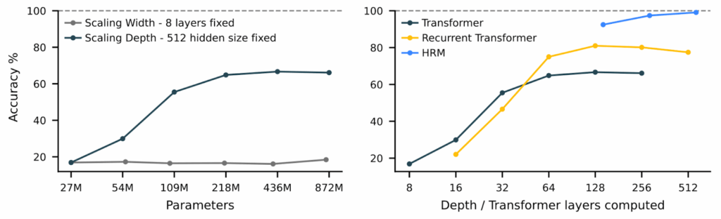
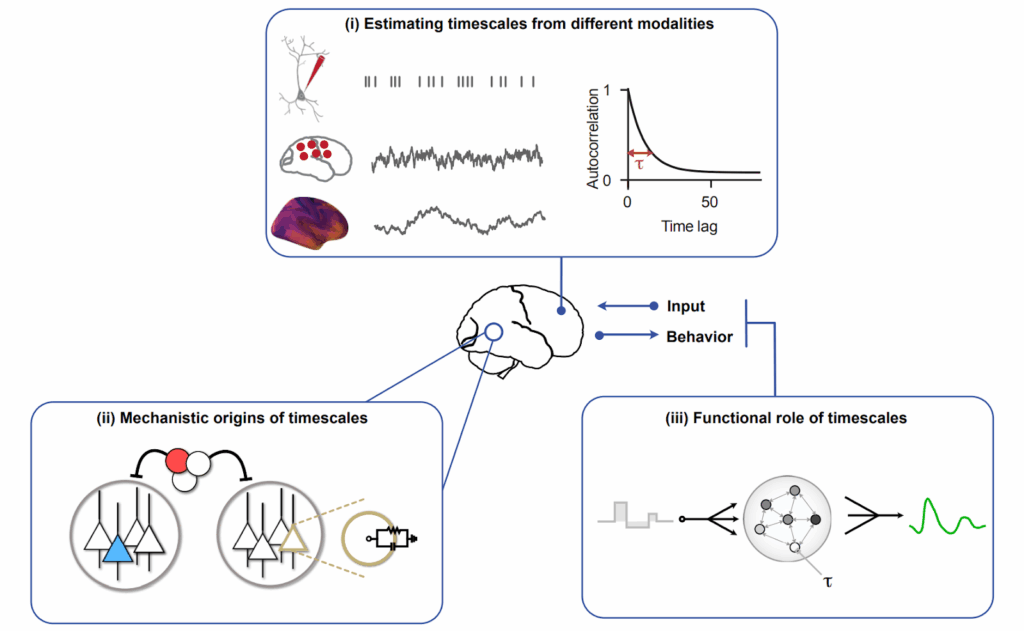
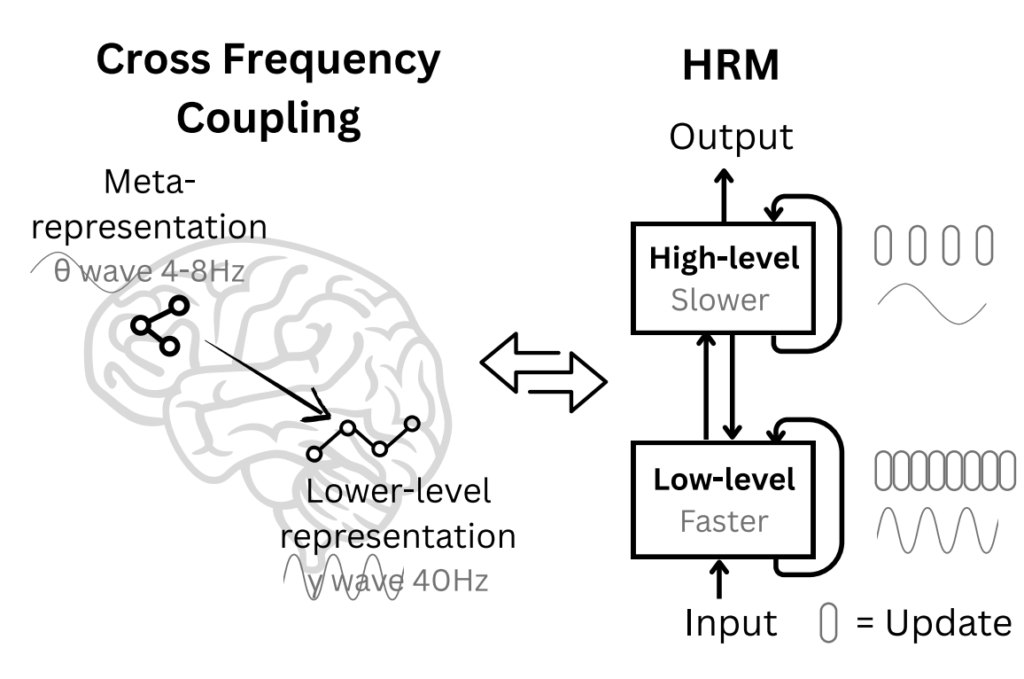
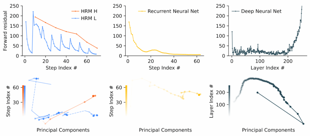
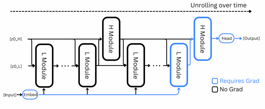
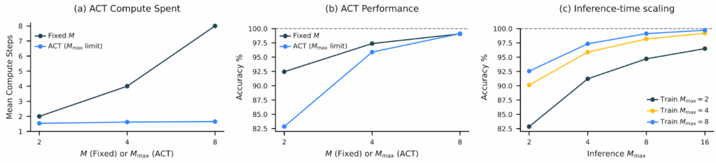
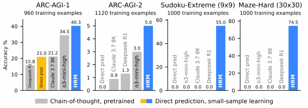
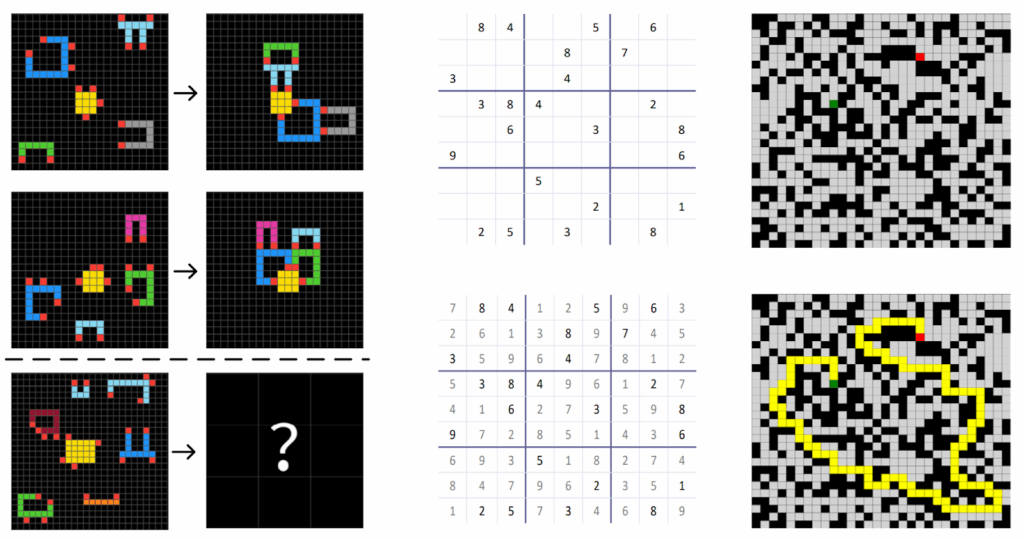
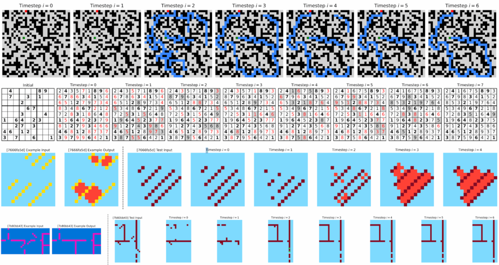
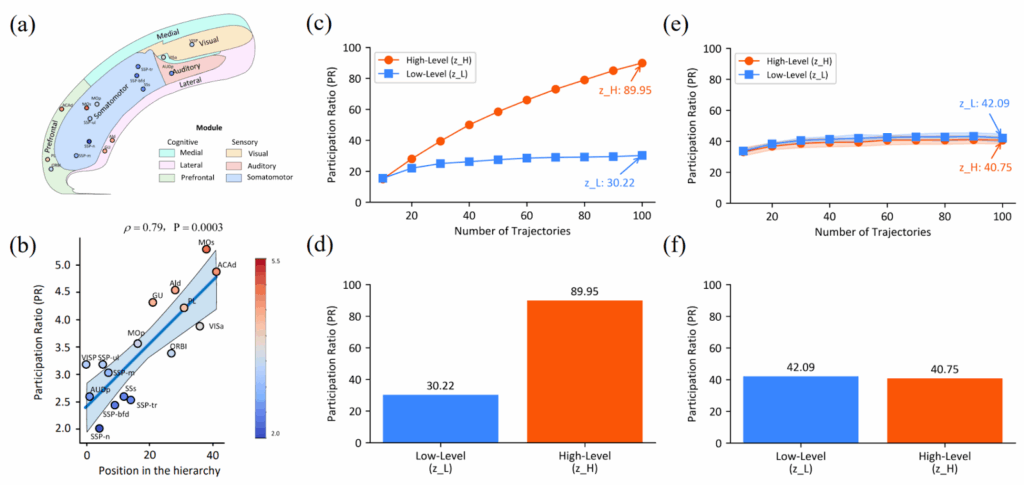


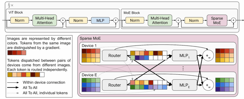
 images composed of
  tokens each, and every token has a representation of dimension
  , so the input is
  ;
; assigns routing weights for every token, so
  is the weight of token
  and expert
  ;
; and assigns each token to its most suitable expert (top-1) if the expert’s buffer is not full, then goes through the rows again and assigns each unassigned token to its top-2 expert if that one’s buffer is not full, and so on.
 for every token based on the maximum routing weight, either just as the maximum weight
  or as the sum of top-k weights for some small
  . Essentially, this assumes that important tokens are those that have clear winners among the experts, while tokens that are distributed uniformly probably don’t matter that much. The BPR algorithm means that the tokens are first ranked according to
  , using the priority scores as a proxy for the priority of allocation. Tokens that have highly uneven distributions of expert probabilities get routed first when experts have bounded capacity.
 that controls the total size of an expert’s buffer. For
  experts, the buffer capacity of each is defined as
 ![\[B_e = \mathrm{round}\left(C\times\frac{kNP}{E}\right),\]](https://blog.sergeynikolenko.ru/wp-content/ql-cache/quicklatex.com-0f39a3d1e582ed514ee17d75e55d8886_l3.svg "Rendered by QuickLaTeX.com")
 , which
  , some tokens will be lost.
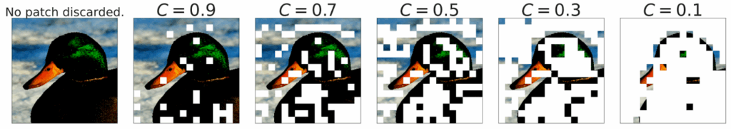
 when V-MoE starts actually dropping tokens (the plots are shown for top-2 routing, i.e.,
  ):
):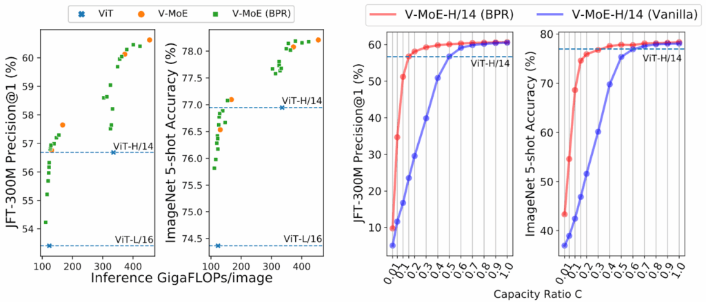
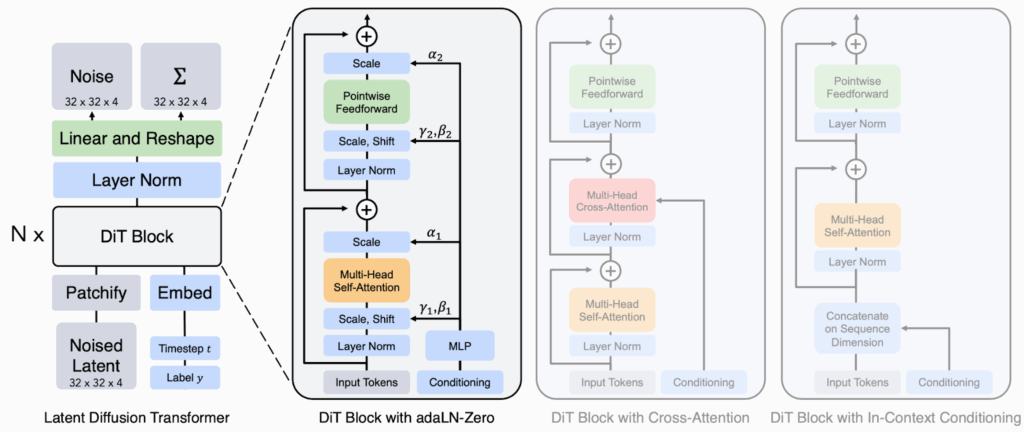
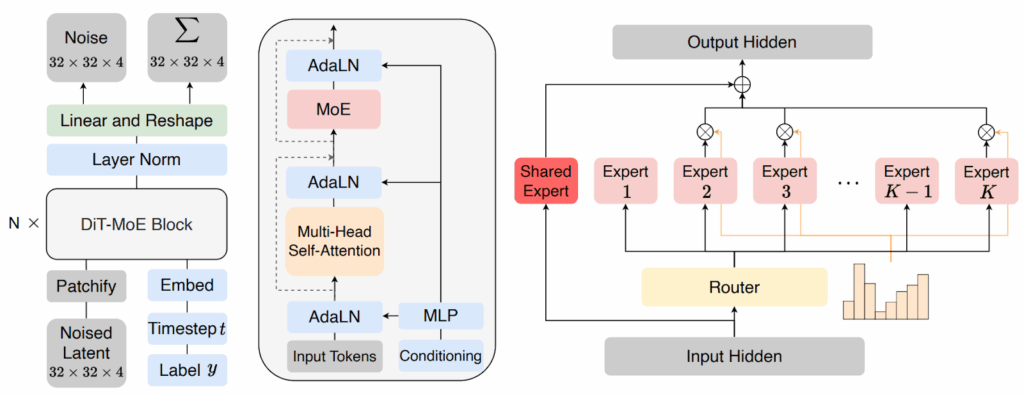
![\[L_{\mathrm{balance}}=\alpha\sum_{i=1}^n\frac{n}{KT}\sum_{t=1}^T\left[\mathrm{Route}(t)=i \right] p(t, i),\]](https://blog.sergeynikolenko.ru/wp-content/ql-cache/quicklatex.com-e08c02c7f69c4e2f3999f344da8853db_l3.svg "Rendered by QuickLaTeX.com")
 is the number of tokens (patches),
  is the number of experts,
 ![\left[\mathrm{Route}(t)=i \right]](https://blog.sergeynikolenko.ru/wp-content/ql-cache/quicklatex.com-faf99bbdbd373015c7c52e6f8b6b088d_l3.svg "Rendered by QuickLaTeX.com") is the indicator function of the fact that token
is the indicator function of the fact that token  routing, and
  is the probability distribution of token
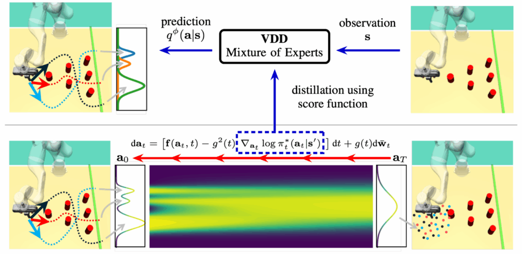
 and a new policy representation
  with parameters
  , the standard variational approach would lead to minimizing the Kullback-Leibler divergence
  , i.e.,
 ![\[\min_\phi \mathrm{KL}(q^\phi(\mathbf{a}|\mathbf{s}')\|\pi(\mathbf{a}|\mathbf{s}')) = \min_\phi{\mathbb E}_{q^\phi(\mathbf{a}|\mathbf{s}')}\left[\log q^\phi(\mathbf{a}|\mathbf{s}') - \log \pi(\mathbf{a}|\mathbf{s}'\right]\]](https://blog.sergeynikolenko.ru/wp-content/ql-cache/quicklatex.com-9dbde984d409722dd18ed728752e4ab9_l3.svg "Rendered by QuickLaTeX.com")
 . This objective then gets more practical by adding two simplifications:
 instead of learning a separate
 ![{\mathbb E}_{q^\phi(\mathbf{a}|\mathbf{s}')}\left[\cdot\right]](https://blog.sergeynikolenko.ru/wp-content/ql-cache/quicklatex.com-326e8bd6911f868124ccd6eddeae212c_l3.svg "Rendered by QuickLaTeX.com") .
.![\[q^\phi(\mathbf{a}|\mathbf{s})=\sum_z q^\xi(\mathbf{z}|\mathbf{s}) q^{\nu_z}(\mathbf{a}|\mathbf{s},\mathbf{z}),\]](https://blog.sergeynikolenko.ru/wp-content/ql-cache/quicklatex.com-401858576ce76e495741e22827bb1a88_l3.svg "Rendered by QuickLaTeX.com")
![\[\nabla_{\mathbf{a}_t}\log \pi_t(\mathbf{a}_t \mid \mathbf{s}) = \mathbf{f}_\theta(\mathbf{a}_t, \mathbf{s}, t).\]](https://blog.sergeynikolenko.ru/wp-content/ql-cache/quicklatex.com-ea15972095219a389d7579a4357e163e_l3.svg "Rendered by QuickLaTeX.com")
 with
with ![\[\nabla_{\phi}\log \pi(\mathbf{a} \mid \mathbf{s}) = \mathbf{f}_\theta(\mathbf{a}, \mathbf{s}, t)\nabla_{\phi}\mathbf{h}^\phi(\mathbf{\epsilon}, \mathbf{s}),\]](https://blog.sergeynikolenko.ru/wp-content/ql-cache/quicklatex.com-affdb2f3ec73d31d167705a9e061fd1a_l3.svg "Rendered by QuickLaTeX.com")
 are reparametrization transformations such that
  for some auxiliary random variable
  ; let’s not get into the specific details of the reparametrization trick here. Overall, this means that we can use variational inference to optimize
  directly without evaluating the likelihoods of
  .
.
![\[J(\phi)=U(\phi,\tilde{q})-\mathbb{E}_{\mu(\mathbf{s})}\mathbb{E}_{q^{\phi}(\mathbf{a}\mid\mathbf{s})}D_{\mathrm{KL}}\bigl(q^{\phi}(z\mid\mathbf{a},\mathbf{s})\mid \tilde{q}(z\mid\mathbf{a},\mathbf{s})\bigr),\]](https://blog.sergeynikolenko.ru/wp-content/ql-cache/quicklatex.com-f635944a98908d0008cf83128ff2c9f0_l3.svg "Rendered by QuickLaTeX.com")
 is an auxiliary distribution and the upper bound is
 ![\[U(\phi,\tilde{q})=\mathbb{E}_{\mu(\mathbf{s})}\mathbb{E}_{q^{\xi}(z\mid\mathbf{s})} \mathbb{E}_{q^{\nu_z}(\mathbf{a}\mid\mathbf{s},z)} \bigl[\log q^{\nu_z}(\mathbf{a}\mid\mathbf{s},z)-\log\pi(\mathbf{a}\mid\mathbf{s}) -\log\tilde{q}(z\mid\mathbf{a},\mathbf{s})\bigr]+\log q^{\xi}(z\mid\mathbf{s})\bigr]\bigr].\]](https://blog.sergeynikolenko.ru/wp-content/ql-cache/quicklatex.com-7502eeb49f14009755d014ed22ad897e_l3.svg "Rendered by QuickLaTeX.com")
![\[U_z^{\mathbf{s}}(\nu_z,\tilde{q})=\mathbb{E}_{q^{\nu_z}(\mathbf{a}\mid\mathbf{s},z)} \bigl[\log q^{\nu_z}(\mathbf{a}\mid\mathbf{s},z)-\log\pi(\mathbf{a}\mid\mathbf{s}) -\log\tilde{q}(z\mid\mathbf{a},\mathbf{s})\bigr]\]](https://blog.sergeynikolenko.ru/wp-content/ql-cache/quicklatex.com-48079c163492bc29f2feea8c0207e488_l3.svg "Rendered by QuickLaTeX.com")
 and state
  .
.
 is obviously an upper bound for
  in two steps:
 individually for every expert with what is basically the standard reverse KL objective but for one expert only;
 :
: ![\[\min_\xi U(\phi,\tilde{q}) = \max_\xi \mathbb{E}_{\mu(\mathbf{s})}\mathbb{E}_{q^{\xi}(z\mid\mathbf{s})}\bigl[\log q^{\xi}(z\mid\mathbf{s}) - U_z^{\mathbf{s}}(\nu_z,\tilde{q})\bigr].\]](https://blog.sergeynikolenko.ru/wp-content/ql-cache/quicklatex.com-c675ababd65cb4b800233c1c0d2c3f1b_l3.svg "Rendered by QuickLaTeX.com")
 is a simple categorical distribution and does not really need the good things we get from variational inference. The main thing about variational bounds is that they let us estimate
  , which has important properties for situations where
  is very complex and
  is much simpler, as is usually the case in machine learning (recall, e.g., my
  , which is basically the maximum likelihood approach. Specifically, the optimization problem for
 ![\[\min_{\xi}\mathbb{E}_{\mu(\mathbf{s})}D_{\mathrm{KL}}\bigl(\pi(\mathbf{a}\mid\mathbf{s})\;\|\;q^{\phi}(\mathbf{a}\mid\mathbf{s})\bigr) =\max_{\xi}\mathbb{E}_{\mu(\mathbf{s})}\mathbb{E}_{\pi(\mathbf{a}\mid\mathbf{s})}\mathbb{E}_{\tilde{q}(z\mid\mathbf{a},\mathbf{s})}\bigl[\log q^{\xi}(z\mid\mathbf{s})\bigr].\]](https://blog.sergeynikolenko.ru/wp-content/ql-cache/quicklatex.com-822ef3d829f21bc9ad2e43e6d9238b5d_l3.svg "Rendered by QuickLaTeX.com")
![\[\min_{\tilde{q}}\mathbb{E}_{\mu(\mathbf{s})}\mathbb{E}_{q^{\phi}(\mathbf{a}|\mathbf{s})}D_{\mathrm{KL}}\left(q^{\phi}(z | \mathbf{a}, \mathbf{s}) \| \tilde{q}(z|\mathbf{a}, \mathbf{s})\right),\]](https://blog.sergeynikolenko.ru/wp-content/ql-cache/quicklatex.com-df2a20da1b7cd587da44b615d1b887b2_l3.svg "Rendered by QuickLaTeX.com")
![\[\tilde{q}(z\mid\mathbf{a},\mathbf{s})=q^{\phi^{\mathrm{old}}}(z\mid\mathbf{a},\mathbf{s}) =\frac{q^{\nu_{z}^{\mathrm{old}}}(\mathbf{a}\mid\mathbf{s},z)\,q^{\xi^{\mathrm{old}}}(z\mid\mathbf{s})}{\sum_{z}q^{\nu_{z}^{\mathrm{old}}}(\mathbf{a}\mid\mathbf{s},z)\,q^{\xi^{\mathrm{old}}}(z\mid\mathbf{s})},\]](https://blog.sergeynikolenko.ru/wp-content/ql-cache/quicklatex.com-489abb17f3eb40b8d881ab04cf51619d_l3.svg "Rendered by QuickLaTeX.com")
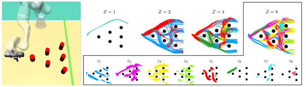
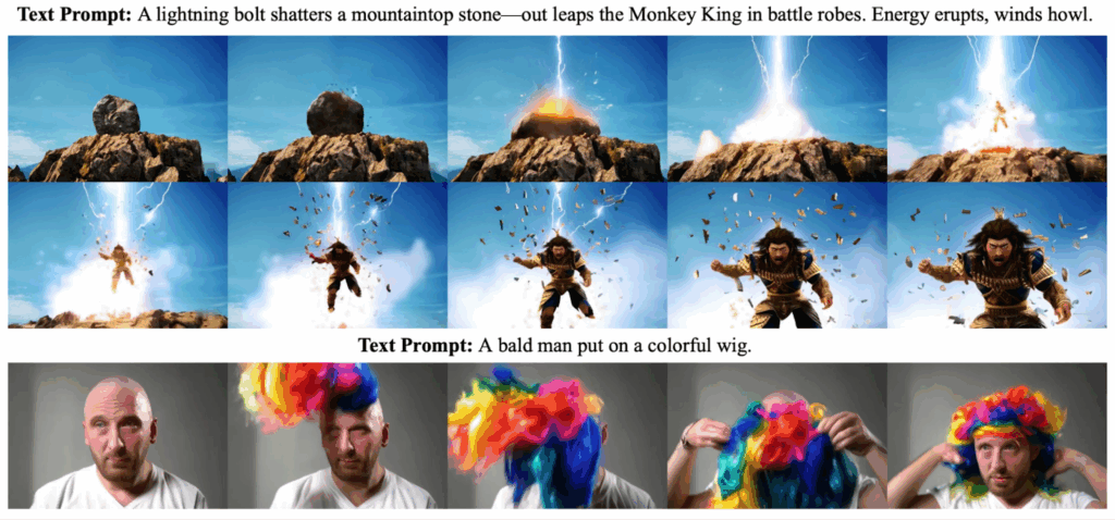
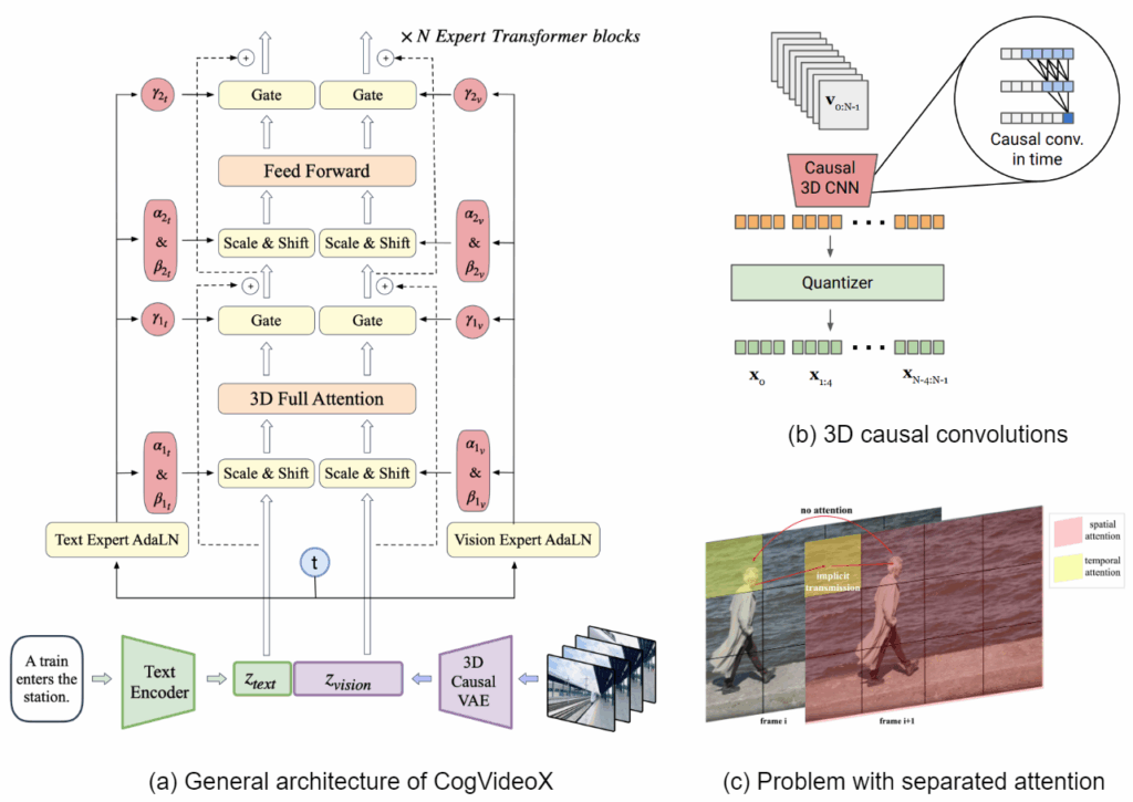
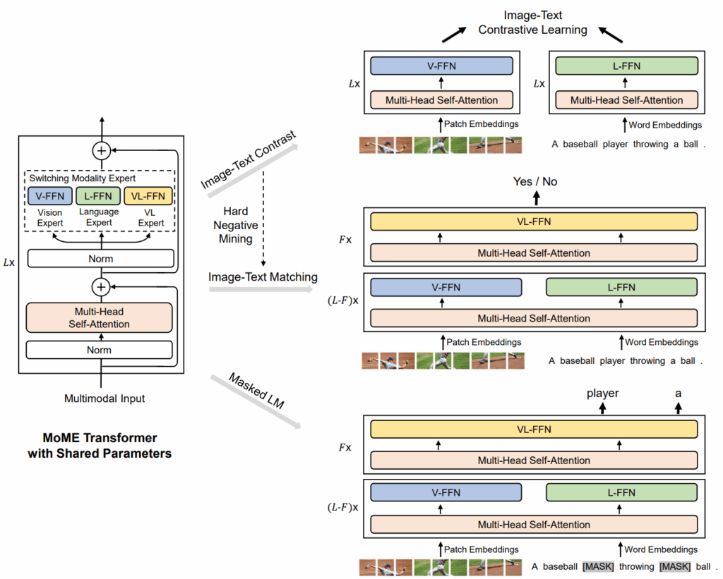
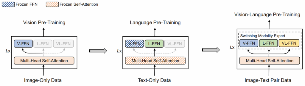
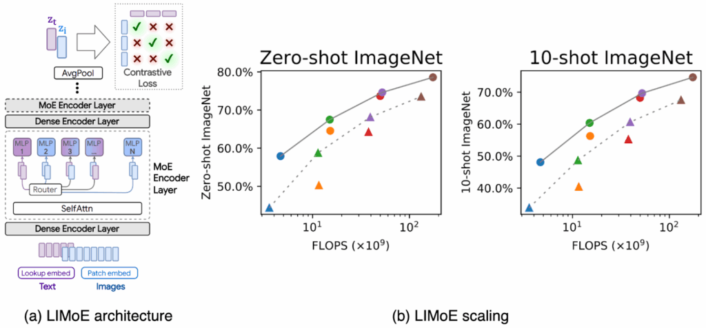
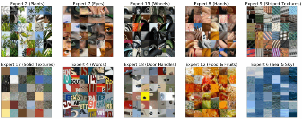
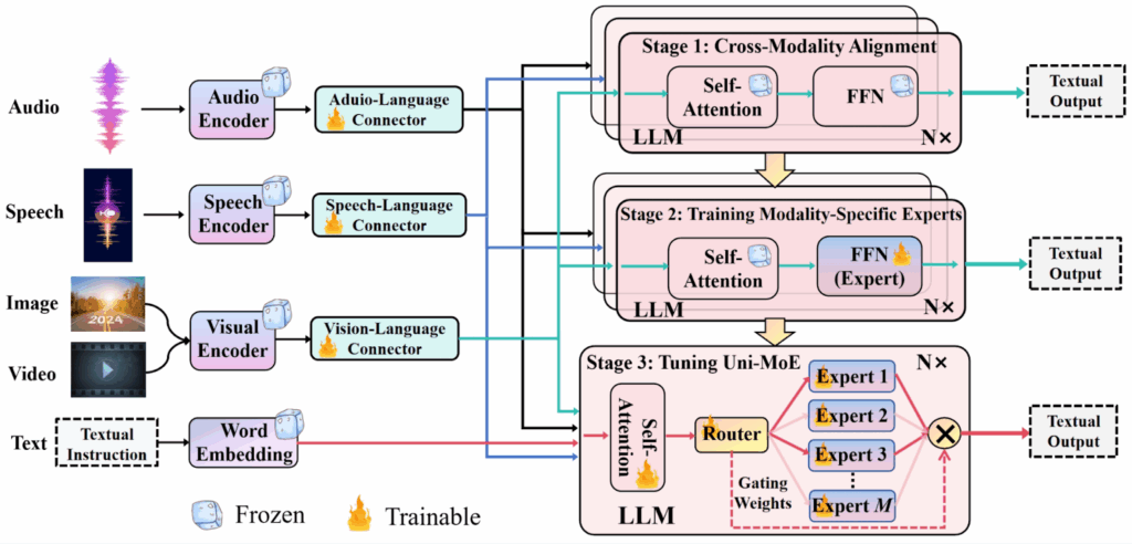
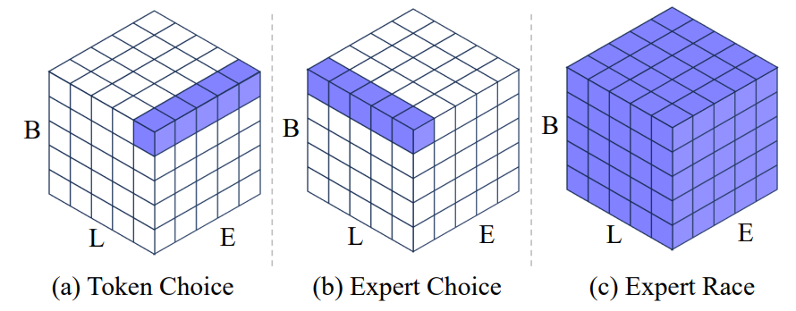
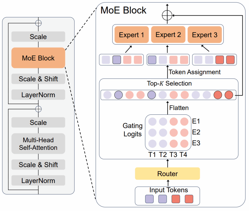
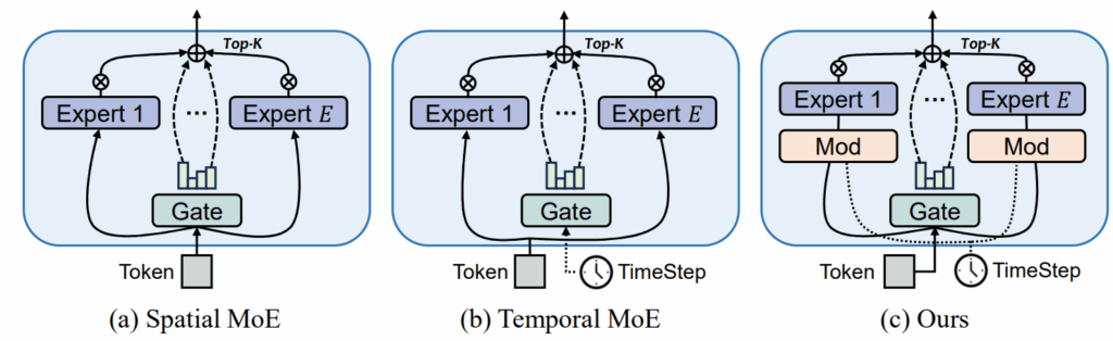
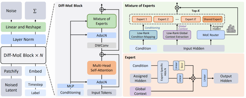
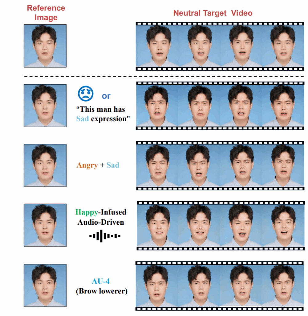
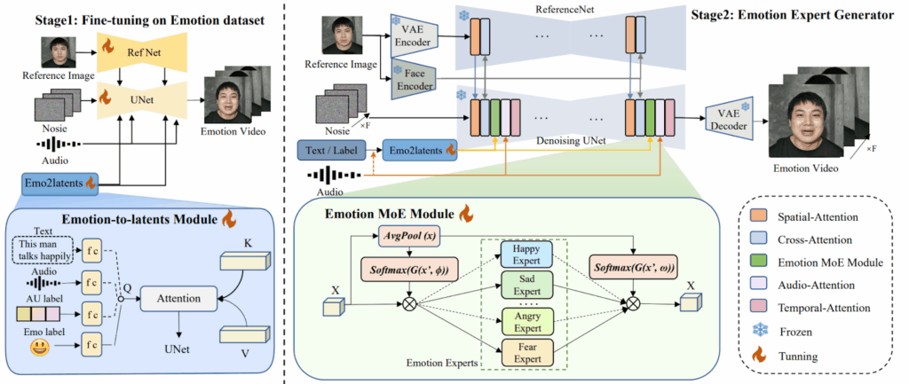
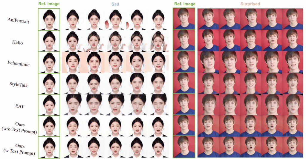
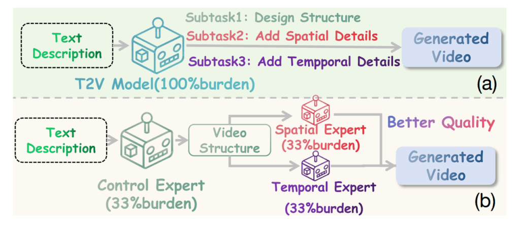
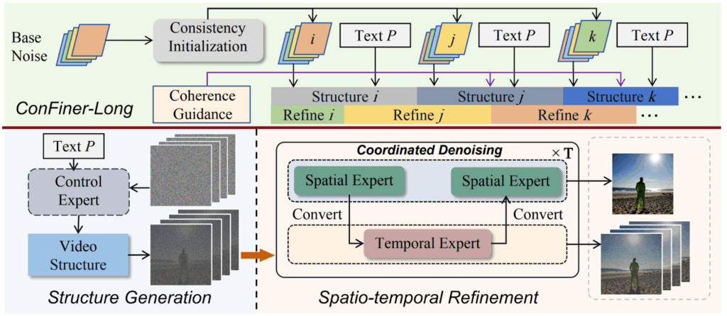
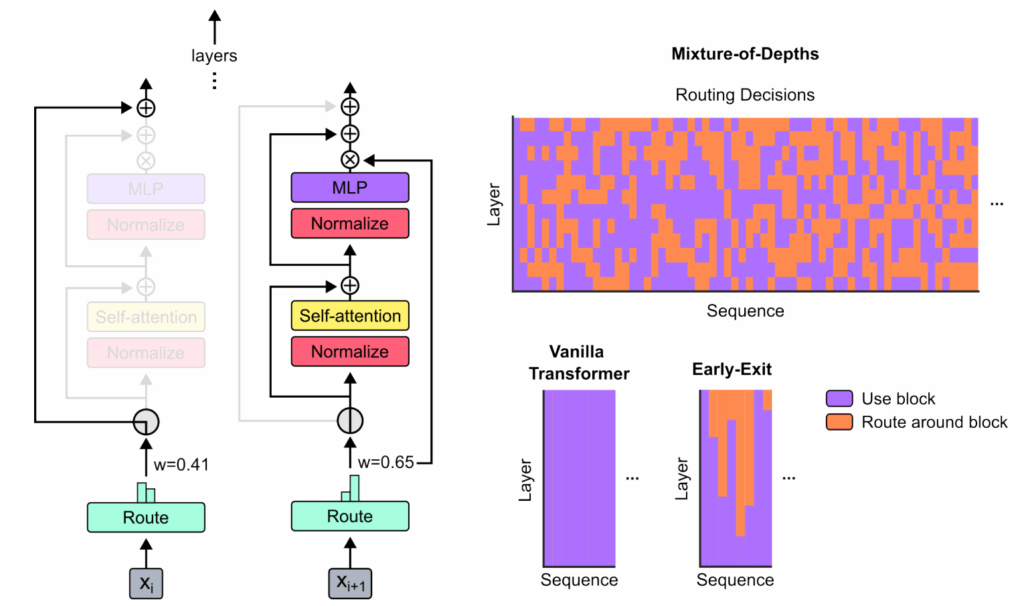
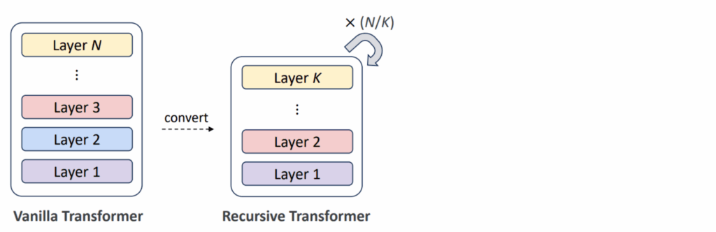
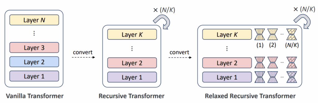
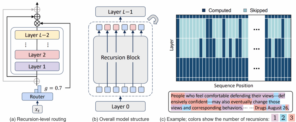
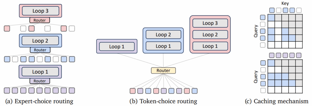


")


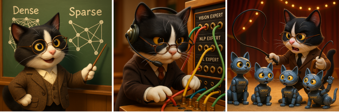

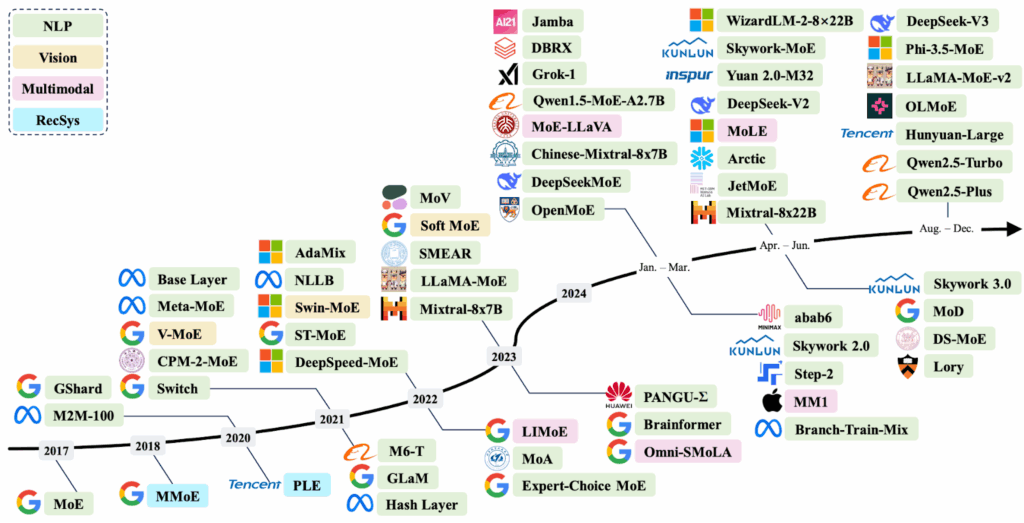
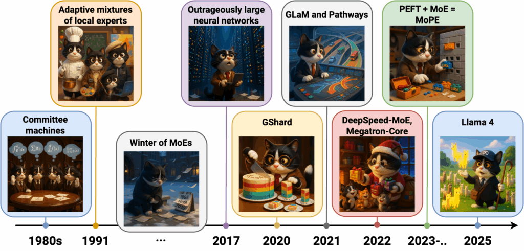
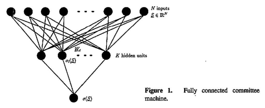
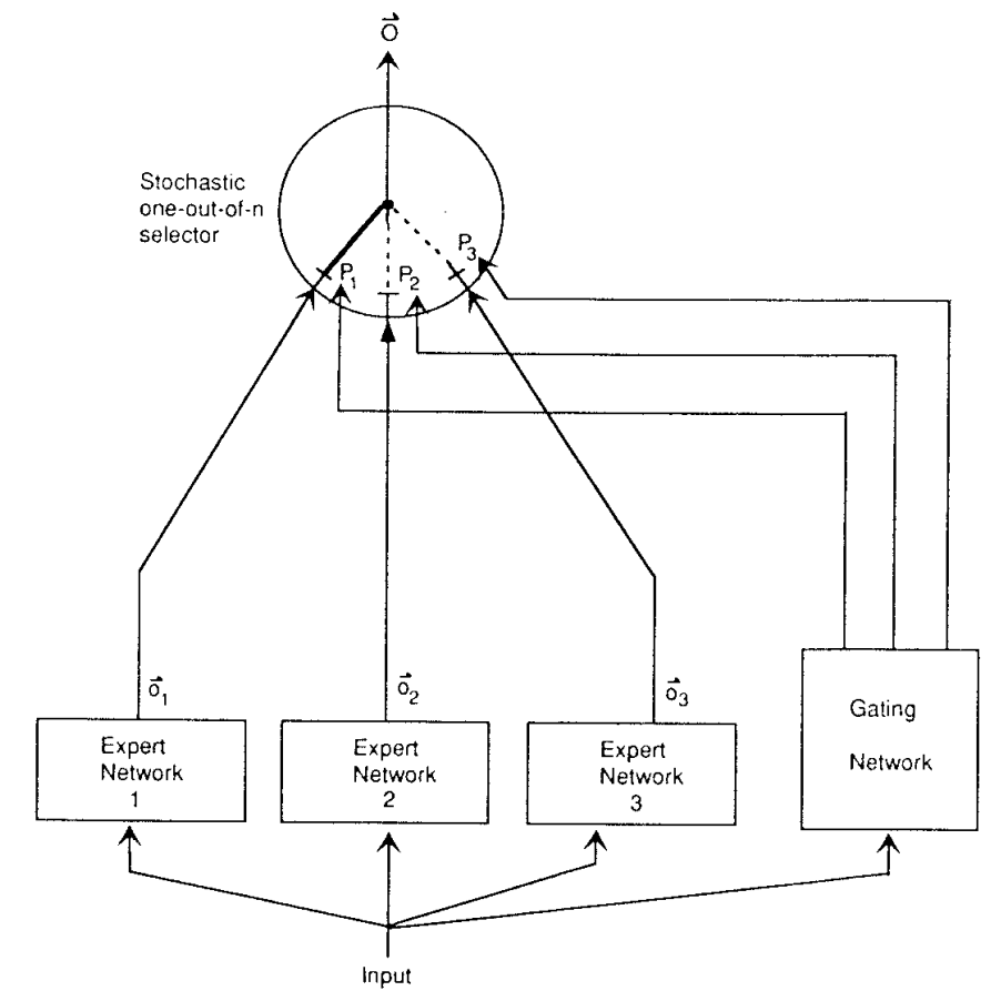

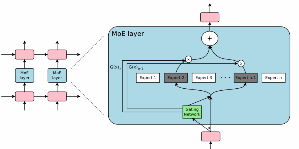
 ,
,  ,
,  input tokens), a self-attention layer took
 ![\[4\cdot L^2\cdot d_{\mathrm{model}} = 4\cdot 128^2 \cdot 1024 \approx 6.7\times 10^7 \text{ FLOPs},\]](https://blog.sergeynikolenko.ru/wp-content/ql-cache/quicklatex.com-045fc0cacda963386dc8e7f723e03491_l3.svg "Rendered by QuickLaTeX.com")
![\[2\cdot L\cdot d_{\mathrm{model}}\cdot d_{\mathrm{FF}} = 2\cdot 128 \cdot 1024 \cdot 8192\approx 2.15\times 10^9 \text{ FLOPs}.\]](https://blog.sergeynikolenko.ru/wp-content/ql-cache/quicklatex.com-103e2668bd5563704a875cbf9977f466_l3.svg "Rendered by QuickLaTeX.com")
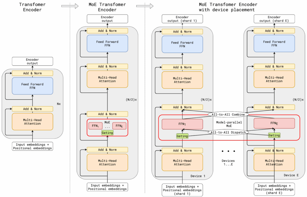

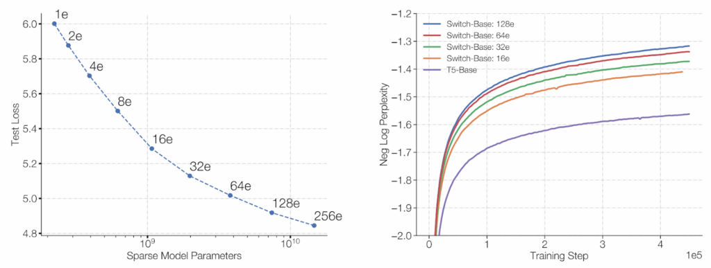

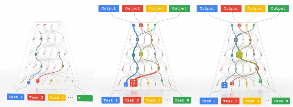
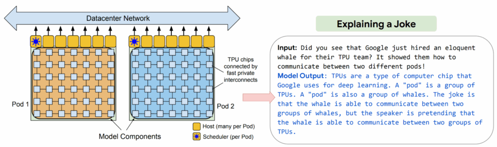
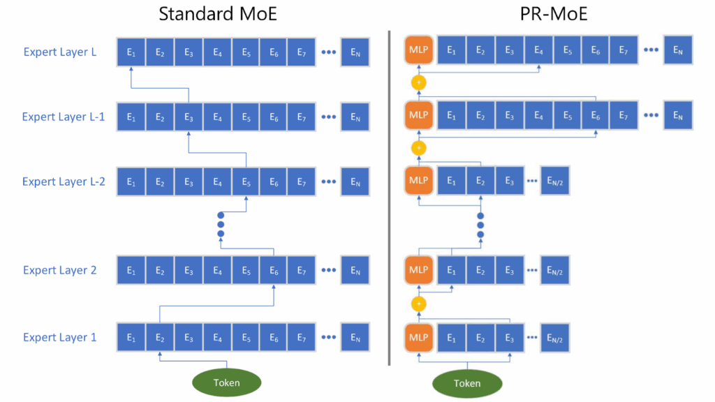
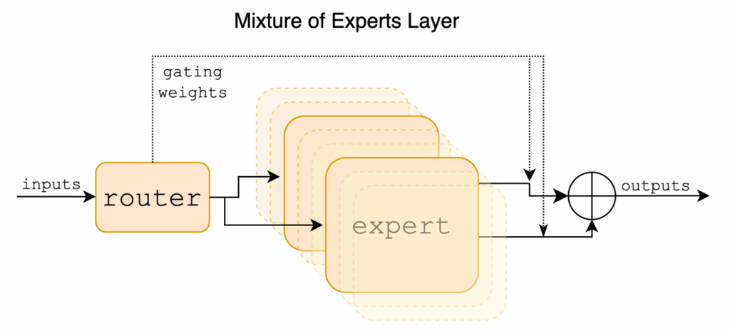
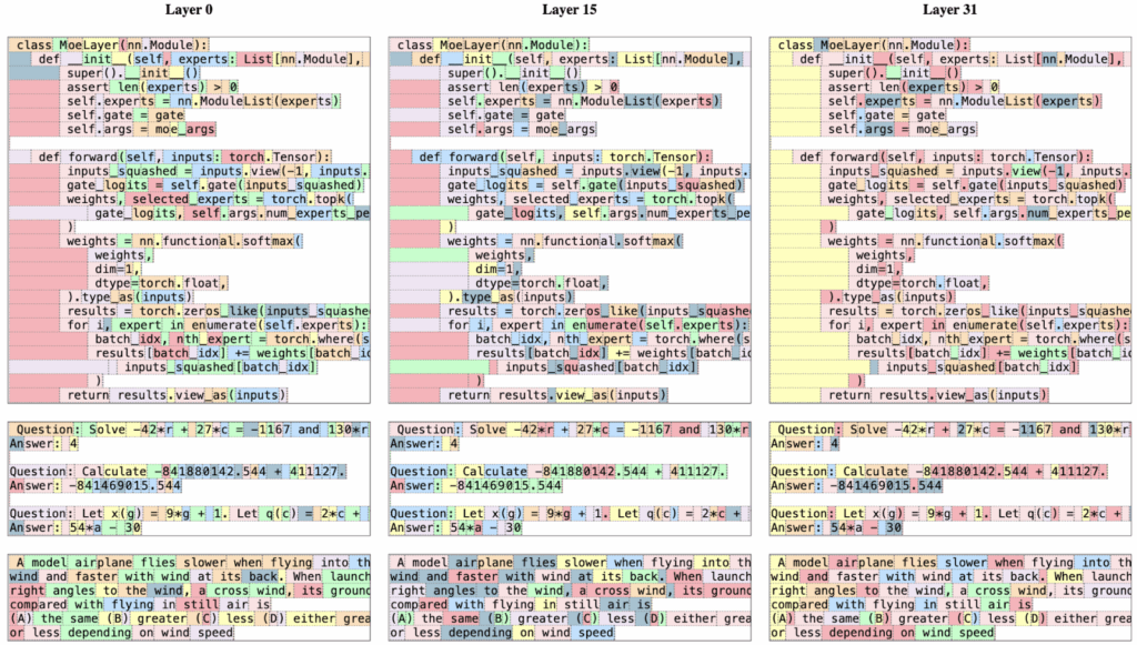
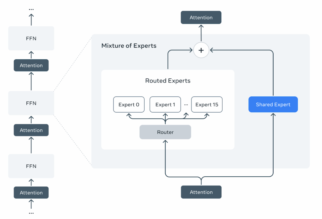
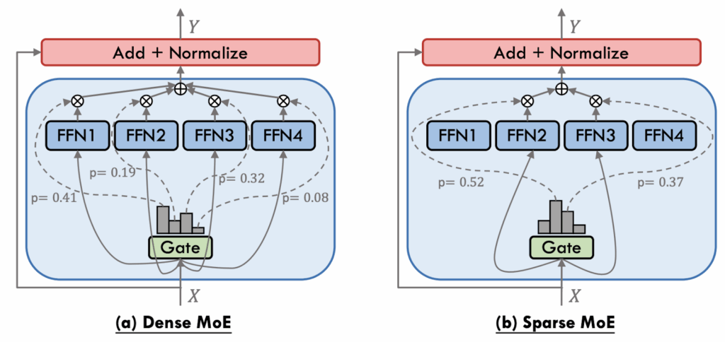
 , where
  are the router’s parameters and
  is the input, and then uses it as softmax scores:
![\[F(\mathbf{x},\boldsymbol{\theta},\mathbf{W})=\sum_{i=1}^n\mathrm{softmax}\left(g(\mathbf{x},\boldsymbol{\theta})\right)\cdot f_i(\mathbf{x},\mathbf{w}_i),\]](https://blog.sergeynikolenko.ru/wp-content/ql-cache/quicklatex.com-f8bcb2f3085edabae172c5cf9dd312a0_l3.svg "Rendered by QuickLaTeX.com")
 are the weights of the experts. A sparse MoE router only leaves the top
 ![\[g_{i,\mathrm{sparse}}(\mathbf{x},\boldsymbol{\theta})=\mathrm{TopK}(\mathbf{g}(\mathbf{x},\boldsymbol{\theta}))_i=\begin{cases} g_i(\mathbf{x},\boldsymbol{\theta}), & \text{if it is in the top }k, \\-\infty, & \text{otherwise}.\end{cases}\]](https://blog.sergeynikolenko.ru/wp-content/ql-cache/quicklatex.com-d73a39d4376fabdb78c9ba49dfa5cb19_l3.svg "Rendered by QuickLaTeX.com")
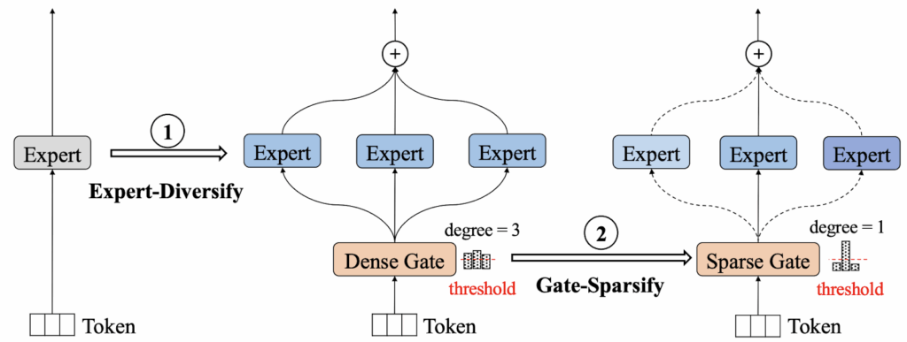
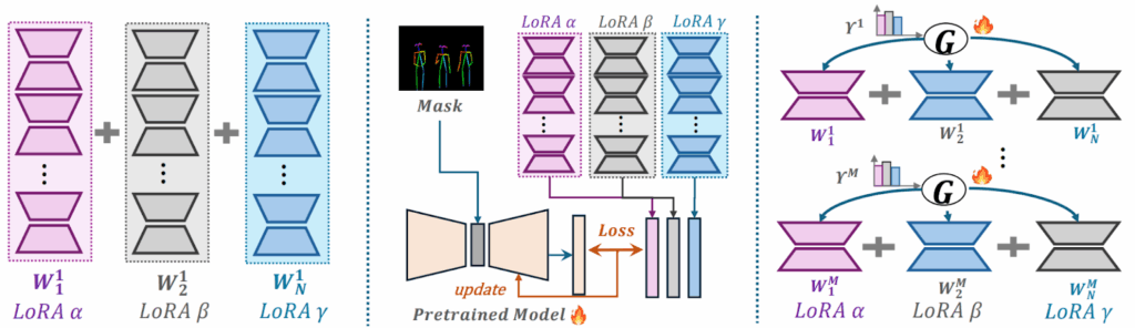
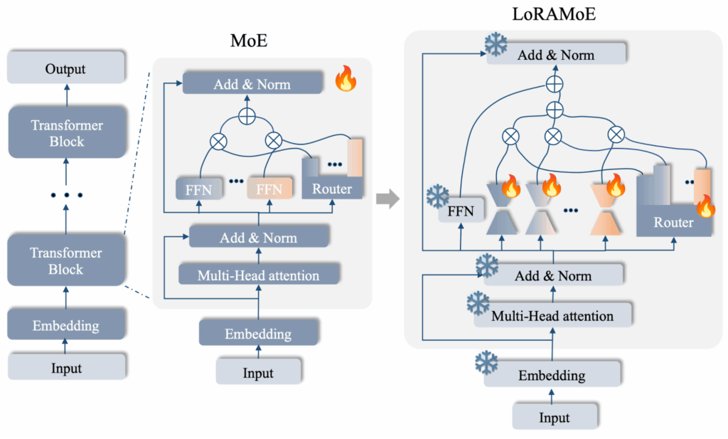
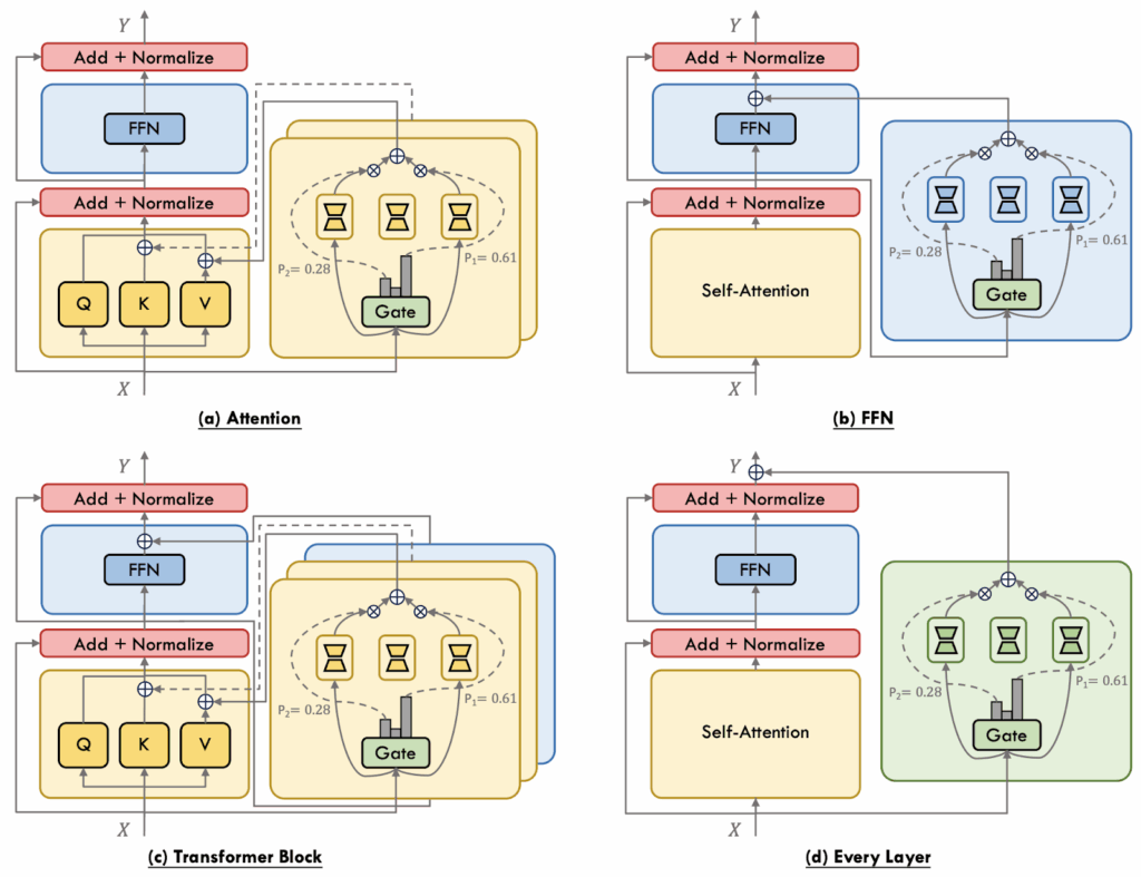


")
")