In the previous post, we posed what we consider the main problem of modern machine learning: increasing appetite for data that cannot be realistically satisfied if current trends persist. This means that current trends will not persist — but what is going to replace them? How can we build machine learning systems at ever increasing scale without increasing the need for huge hand-labeled datasets? Today, we consider one possible answer to this question: one-shot and zero-shot learning.
How can Face Recognition Work?
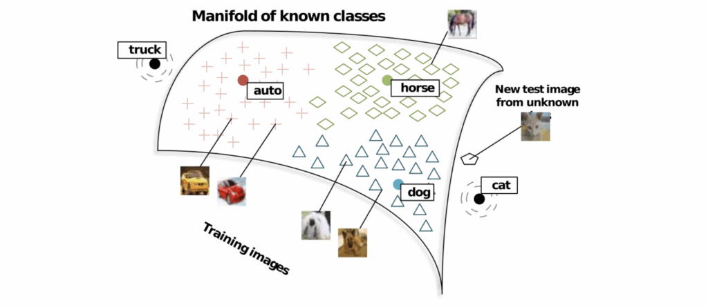
Consider a face recognition system. For simplicity, let’s assume that our system is a face classifier so that we do not need to worry about object detection, bounding box proposals and all that: the face is already pre-cut from a photo, and all we have to do is recognize the person behind that face.
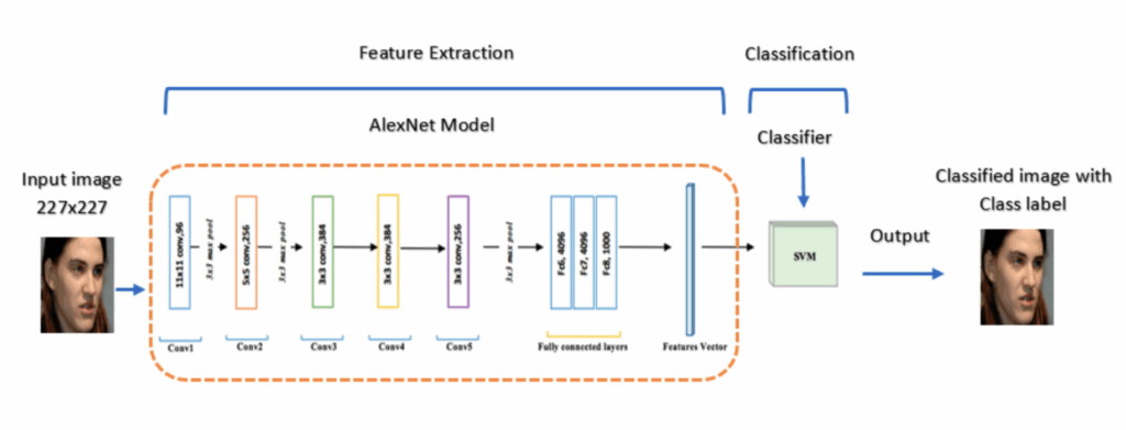
A regular image classifier consists of a feature extraction network followed by a classification model; in deep learning, the latter is usually very simple, and feature extraction is the interesting part. Like this (image source):
So now we train this classifier on our large labeled dataset of faces, and it works great. But wait: where do the labeled samples come from? Sure, we can assume that a large labeled dataset of some human faces is available, but a face recognition system needs to do more: while it’s okay to require a large dataset for pretraining, a live model needs to be able to recognize new faces.
How is this use case supposed to work? Isn’t the whole premise of training machine learning models that you need a lot of labeled data for each class of objects you want to recognize? But if so, how can a face recognition system hope to recognize a new face when it usually has at most a couple of shots for each new person?
One-Shot Learning via Siamese Networks
The answer is that face recognition systems are a bit different from regular image classifiers. Any machine learning system working with unstructured data (such as photos) is basically divided into two parts: feature extraction, the part that converts an image into a (much smaller) set of numbers, often called an embedding or a latent code, and a model that uses extracted features to actually solve the problem. Deep learning is so cool because neural networks can learn to be much better at feature extraction than anything handcrafted that we had been able to come up with. In the AlexNet-based classifier shown above, the hard part was the AlexNet model that extracts features, and the classifier can be any old model, usually simple logistic regression.
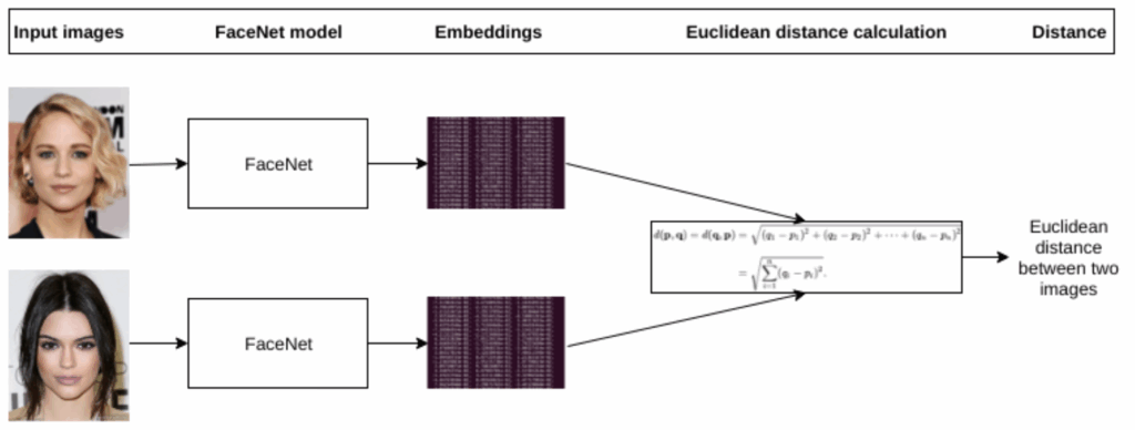
To get a one-shot learning system, we need to use the embeddings in a different way. In particular, modern face recognition systems learn face embeddings with a different “head” of the network and different error functions. For example, FaceNet (Schroff et al., 2015) learns with a modification of the Siamese network approach, where the target is not a class label but rather the distances or similarities between face embeddings. The goal is to learn embeddings in such a way that embeddings of the same face will be close together while embeddings of different faces will be clearly separated, far from each other (image source):
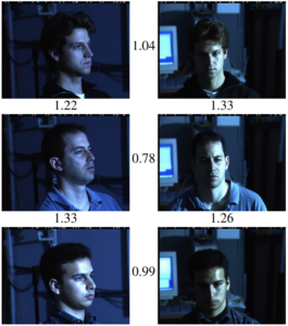
The “FaceNet model” in the picture does feature extraction. Then to compute the error function you compute the distance between two embedding vectors. If the two input faces belong to the same person, you want the embedding vectors to be close together, and if they are different people, you want to push the embeddings together. There is still some way to go from this basic idea before we have a usable error function, but this will suffice for a short explanation. Here is how FaceNet works as a result; in the picture below, the numbers between photos of faces correspond to the distances between their embedding vectors (source):
Note that the distances between two photos of the same guy are consistently smaller than distances between photos of different people, even though in terms of pixels, composition, background, lighting, and basically everything else except for human identity the pictures in the columns are much more similar than pictures in the rows.
Now, after you have trained a model with these distance-based metrics in mind, you can use the embeddings to do one-shot learning itself. Assuming that a new face’s embedding will have the same basic properties, we can simply compute the embedding for a new person (with just a single photo as input!) and then do classification by looking for nearest neighbors in the space of embeddings.
Zero-Shot Learning and Generative Models
We have seen a simplified but relatively realistic picture of how one-shot learning systems work. But one can go even further: what if there is no data at all available for a new class? This is known as zero-shot learning.
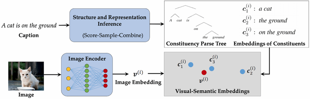
The problem sounds impossible, and it really is: if all you know are images from “class 1” and “class 2”, and then you are asked to distinguish between “class 3” and “class 4”, no amount of machine learning can help you. But real life does not work this way: we usually have some background knowledge about the new classes even if we don’t have any images. For example, when we are asked to recognize a “Yorkshire terrier”, we know that it’s a kind of dog, and maybe we even have its verbal description, e.g., from Wikipedia. With this information, we can try to learn a joint embedding space for both class names and images, and then use the same nearest neighbors approach but look for the nearest label embedding rather than other images (which we have none for a new class). Here is how Socher et al. (2013) illustrate this approach:
Naturally, this won’t give you the same kind of accuracy as training on a large labeled set of images, but systems like this are increasingly successful.
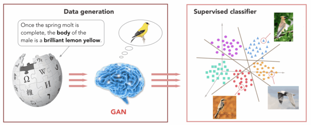
Many zero-shot learning models use generative models and adversarial architectures. One of my favorite examples is a (more) recent paper by Zhu et al. (2018) that uses a generative adversarial network (GAN) to “hallucinate” images of new classes by their textual descriptions and then extracts features from these hallucinated images:
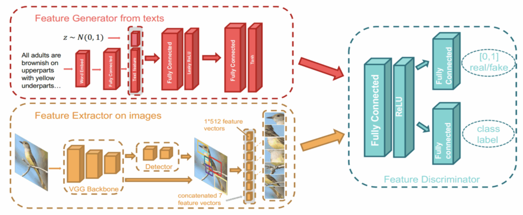
The interesting part here is that they do not need to solve the extremely complex and fragile problem of generating high-resolution images of birds that only the very best of GANs can do (such as, e.g., BigGAN and its successors). They train a GAN to generate not images but rather feature vectors, those very same joint embeddings, and this is, of course, a much easier problem. Zhu et al. use a standard VGG architecture to extract features from images and train a conditional GAN to generate such feature vectors given a latent vector of textual features extracted from the description:
As a result, you can do extremely cool things like zero-shot retrieval: doing an image search against a database without any images corresponding to your query. Given the name of a bird, the system queries Wikipedia, extracts a textual description, uses the conditional GAN to generate a few vectors of visual features for the corresponding bird, and then looks for its nearest neighbors in the latent space among the images in the database. The results are not perfect but still very impressive:
Note, however, that one- and zero-shot learning still require large labeled datasets. The difference is that we don’t need a lot of images for new classes any more. But the feature extraction network has to be trained on similar labeled classes: a zero-shot approach won’t work if you train it on birds and then try to look for a description of a chair. Until we have an uber-network trained on every kind of images possible (and believe me, we still have quite a way to go before Skynet enslaves the human race), this is still a data-intensive approach, although restrictions on what kind of data to use are relaxed.
Conclusion
In this post, we have seen how one-shot and zero-shot learning can help by drastically reducing the need for labeled datasets in the context of:
either adding new classes to an existing machine learning model (one-shot learning)
or transforming data from one domain, where it might be plentiful, to another, e.g., mapping textual descriptions to images (zero-shot learning).
But we have also seen that all of these approaches still need a large dataset to begin with. For exampe, a one-shot learning model for human faces needs to have a large labeled dataset of human faces to work, and only then we can add new people with a single photo. A zero-shot model that can hallucinate pictures of birds based on textual descriptions needs a lot of descriptions paired with images before it is able to do its zero-shot magic.
This is, of course, natural. Moreover, it is quite possible that at some point of AI development we will already have enough labeled data to cover entire fields such as computer vision or sound processing, extending their capabilities with one-shot and zero-shot architectures. But while we are not at that point yet, and there is no saying whether we can reach it in the near future, we need to consider other methods for alleviating the data problem. In the next installment of this series, we will see how unlabeled data can be used in this regard.
Today, we are kicking off the Synthesis AI blog. In these posts, we will speak mostly about our main focus, synthetic data, that is, artificially created data used to train machine learning models. But before we begin to dive into the details of synthetic data generation and use, I want to start with the problem setting. Why do we need synthetic data? What is the problem and are there other ways to solve it? This is exactly what we will discuss in the first series of posts.
Structure of a Machine Learning Project
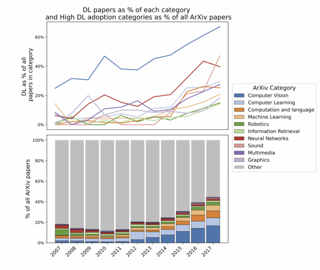
Machine learning is hot, and it has been for quite some time. The field is growing exponentially fast, new models and new papers appear every week, if not every day. Since the deep learning revolution, for about a decade deep learning has been far outpacing other fields of computer science and arguably even science in general. Here is a nice illustration from Michael Castelle’s excellent post on deep learning:
It shows how deep learning is taking up more and more of the papers published on arXiv (the most important repository of computer science research); the post was published in 2018, but trust me, the trend continues to this day.
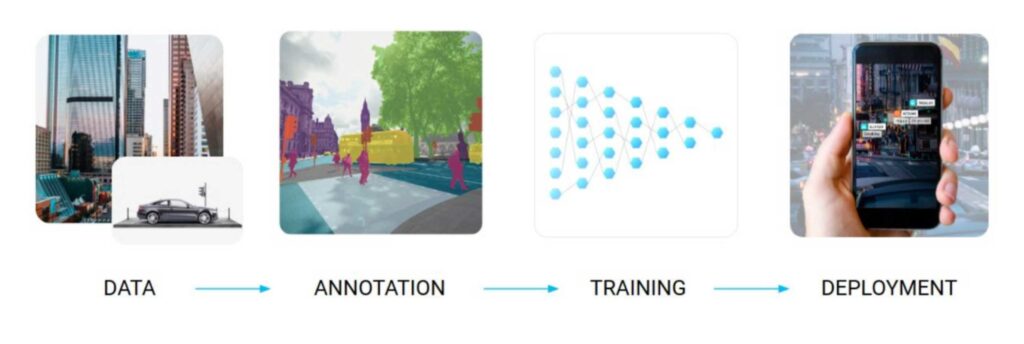
Still, the basic pipeline of using machine learning for a given problem remains mostly the same, as shown in the teaser picture for this post:
first, you collect raw data related to your specific problem and domain;
second, the data has to be labeled according to the problem setting;
third, machine learning models train on the resulting labeled datasets (and validate their performance on subsets of the datasets set aside for testing);
fourth, after you have the model you need to deploy it for inference in the real world; this part often involves deploying the models in low-resource environments or trying to minimize latency.
The vast majority of the thousands of papers published in machine learning deal with the “Training” phase: how can we change the network architecture to squeeze out better results on standard problems or solve completely new ones? Some deal with the “Deployment” phase, aiming to fit the model and run inference on smaller edge devices or monitor model performance in the wild.
Still, any machine learning practitioner will tell you that it is exactly the “Data” and (for some problems especially) “Annotation” phases that take upwards of 80% of any real data science project where standard open datasets are not enough. Will these 80% turn into 99% and become a real bottleneck? Or have they already done so? Let’s find out.
Are Machine Learning Models Hitting a Wall?
I don’t have to tell you how important data is for machine learning. Deep learning is especially data-hungry: usually you can achieve better results with “classical” machine learning techniques on a small dataset, but as the datasets grow, the flexibility of deep neural networks, with their millions of weights free to choose any kind of features to extract, starts showing. This was a big part of the deep learning revolution: even apart from all the new ideas, as the size of available datasets and the performance of available computational devices grew neural networks began to overcome the competition.
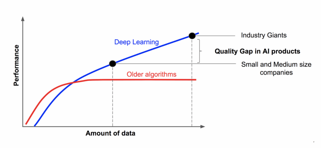
By now, large in-house datasets are a large part of the advantage that industry giants such as Google, Facebook, or Amazon have over smaller companies (image taken from here):
I will not tell you how to collect data: it is very problem-specific and individual for every problem domain. However, data collection is only the first step; after collection, there comes data labeling. This is, again, a big part of what separates industry giants from other companies. More than once, I had big companies tell me that they have plenty of data; and indeed, they had collected terabytes of important information… but the data was not properly curated, and most importantly, it was not labeled, which immediately made it orders of magnitude harder to put to good use.
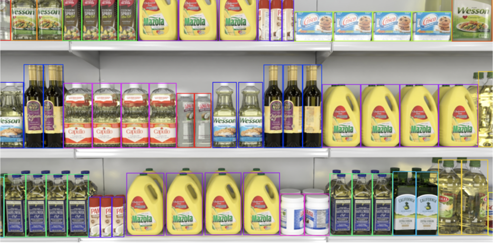
Throughout this series, I will be mostly taking examples from computer vision. For computer vision problems, the labeling required is often very labor-intensive. Suppose that you want to teach a model to recognize and count retail items on a supermarket shelf, a natural and interesting idea for applying computer vision in retail; here at Synthesis AI, we have had plenty of experience with exactly this kind of projects.
Since each photo contains multiple objects of interest (actually, a lot, often in the hundreds), the basic computer vision problem here is object detection, i.e., drawing bounding boxes around the retail items. To train the model, you need a lot of photos with labeling like this:
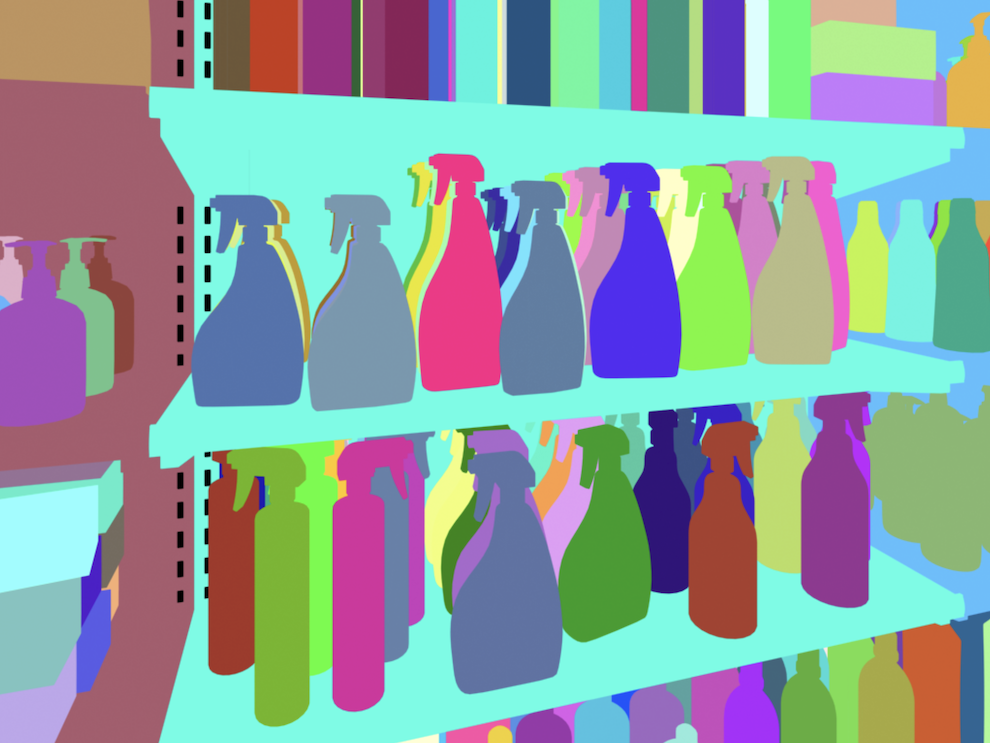
If we also needed to do segmentation, i.e., distinguishing the silhouettes of items, we would need a lot of images with even more complex labeling, like this:
Imagine how much work it is to label a photo like this by hand! Naturally, people have developed tools to help partially automate the process. For example, a labeling tool will suggest a segmentation done by some general-purpose model, and you are only supposed to fix its mistakes. But it may still take minutes per photo, and the training set for a standard segmentation or object detection model should have thousands of such photos. This adds up to human-years and hundreds of thousands, if not millions, of dollars spent on labeling only.
There exist large open datasets for many different problems, segmentation and object detection included. But as soon as you need something beyond the classes and conditions that are already well covered in these datasets, you are out of luck; ImageNet does have cows, but not shot from above with a drone.
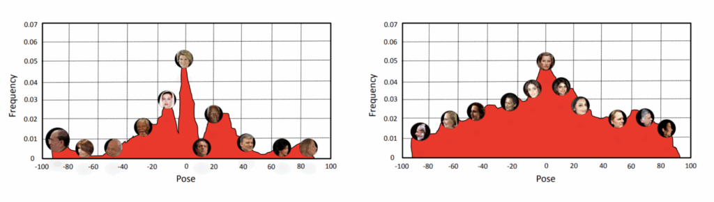
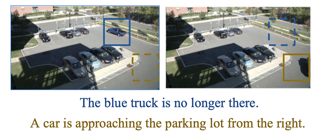
And even if the dataset appears to be tailor-made for your problem, it can contain dangerous biases. For example, suppose you want to recognize faces, a classic problem with large-scale datasets freely available. But if you want to recognize faces “in the wild”, you need a dataset that covers all sorts of rotations for the faces, while standard datasets mostly consist of frontal pictures. In the picture below, taken from (Zhao et al., 2017), on the left you see the distribution of face rotations in IJB-A (a standard open large-scale face recognition dataset), and the picture on the right shows how it probably should look if you really want your detection to be pose-invariant:
To sum up: current systems are data-intensive, data is expensive, and we are hitting the ceiling of where we can go with already available or easily collectible datasets, especially with complex labeling.
Possible Solutions
So what’s next? How can we solve the data problem? Is machine learning heading towards a brick wall? Hopefully not, but it will definitely take additional efforts. In this series of posts, we will find out what researchers are already doing. Here is a tentative plan for the next installments, laid out according to different approaches to the data problem:
first, we will discuss models able to train on a very small number of examples or even without any labeled training examples at all (few-shot, one-shot, and even zero-shot learning); usually, few-shot and one-shot models learn a representation of the input in some latent space, while zero-shot models rely on some different information modality, e.g., zero-shot retrieval of images based on textual descriptions (we’ll definitely talk about this one, it’s really cool!);
next, we will see how unlabeled data can be used to pretrain or help train models for problems that are usually trained with labeled datasets; for example, in a recent work Google Brain researchers Xie et al. (2019) managed to improve ImageNet classification performance (not an easy feat in 2019!) by using as additional information a huge dataset of unlabeled photos; such approaches require a lot of computational resources, “trading” computation for data;
and finally, we will come to the main topic of this blog: synthetic data; for instance, computer vision problems can benefit from pixel-perfect labeling that comes for free with 3D renderings of synthetic scenes (Nikolenko, 2019); but this leads to an additional problem: domain transfer for models trained on synthetic data into the real domain.
Let’s summarize. We have seen that modern machine learning is demanding larger and larger datasets. Collecting and especially labeling all this data becomes a huge task that threatens future progress in our field. Therefore, researchers are trying to find ways around this problem; next time, we will start looking into these ways!
Welcome to the final, fifth part of my review for the ACL 2019 conference! You can find previous installments here: Part 1, Part 2, Part 3, Part 4. Today we proceed to the workshop day. Any big conference is accompanied by workshops. While some people may think that workshops are “lower status”, and you submit to a workshop if you assume you have very little chance to get the paper accepted to the main conference, they are in fact very interesting events that collect wonderful papers around a single relatively narrow topic.
The workshop that drew my attention was the Second Storytelling Workshop, a meeting devoted to a topic that sounded extremely exciting: how do you make AI write not just grammatically correct text but actual stories? This sounded wonderful in theory but in practice, I didn’t really like the papers. I hate to criticize, but somehow it all sounded like ad hoc methods that might bring incremental improvements but cannot bring us close to the real thing. So, for the afternoon session, I went to the NLP for Conversational AI Workshop; there, I was guaranteed some great talks because nearly all of them were invited talks, which are usually delivered by eminent researchers and contain survey-like expositions of their work.
So, for today’s final installment on ACL, I will discuss only two talks from the conference. First, we will work our way through the invited talk at the NLP for Conversational AI Workshop by Professor Yejin Choi. And then we will look at a sample paper from the Second Storytelling Workshop — let’s see if you agree with my evaluation.
The Curious Case of Degenerate Neural Conversation
This was an invited talk by Professor Yejin Choi from the University of Washington (see this link for the slides; all pictures below are taken from there), where she discussed what is missing from all current neural models for natural language generation.
She started by recalling the Alexa Prize that they won in 2017, but even their winning solution was not an end-to-end neural model. Why not? Humans understand language through their understanding of the world. Neural language models lack any knowledge of the world but generate text based on statistical correlations (okay, it’s a bit more complicated but still). The main problem in text generation and conversational AI is to bridge this gap. On the surface, this can be done by introducing long-term coherence to neurally generated text. But deep down, what we really want is to give the models some kind of common-sense understanding about people and the world around us. This is a huge problem and Professor Choi and her group are actually working towards this goal, but it is still very far from a successful resolution.
First, let’s begin with a look at the OpenAI GPT2 model with their famous unicorn example.
Seed (text provided for the model): In a shocking finding, scientist discovered a herd of unicorns living in a remote, previously unexplored valley, in the Andes Mountains. Even more surprising to the researchers was the fact that the unicorns spoke perfect English.
Generated text (continuation, best of 10 tries): The scientist named the population, after their distinctive horn, Ovid’s Unicorn. These four-horned, silver-white unicorns were previously unknown to science.
Now, after almost two centuries, the mystery of what sparked this odd phenomenon is finally solved.
Dr. Jorge Pérez, an evolutionary biologist from the University of La Paz, and several companions, were exploring the Andes Mountains when they found a small valley, with no other animals or humans. Pérez noticed that the valley had what appeared to be a natural fountain, surrounded by two peaks of rock and silver snow.
Pérez and the others then ventured further into the valley. “By the time we reached the top of one peak, the water looked blue, with some crystals on top,” said Pérez.
Pérez and his friends were astonished to see the unicorn herd. These creatures could be seen from the air without having to move too much to see them — they were so close they could touch their horns.
While examining these bizarre creatures the scientists discovered that the creatures also spoke some fairly regular English. Pérez stated, “We can see, for example, that they have a common ‘language,’ something like a dialect or dialectic.”
Dr. Pérez believes that the unicorns may have originated in Argentina, where the animals were believed to be descendants of a lost race of people who lived there before the arrival of humans in those parts of South America.
While their origins are still unclear, some believe that perhaps the creatures were created when a human and a unicorn met each other in a time before human civilization. According to Pérez, “In South America, such incidents seem to be quite common.”
However, Pérez also pointed out that it is likely that the only way of knowing for sure if unicorns are indeed the descendants of a lost alien race is through DNA. “But they seem to be able to communicate in English quite well, which I believe is a sign of evolution, or at least a change in social organization,” said the scientist.
We had never seen neurally generated text of this quality, but note that it still took 10 tries to generate, and there was some random sampling that led to these 10 different tries. If, however, we use beam search instead of random sampling for generation, we get a much stranger text that soon degenerates into a closed loop:
Why does neural text, even in the very best model, degenerate like this? Let’s try different approaches on another example. If we choose the best hypothesis every time, we once again quickly arrive at a closed loop:
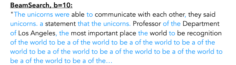
Beam search, which looks ahead for a few words, should perform better, right? But in this case, if we use beam search, we only make things worse:
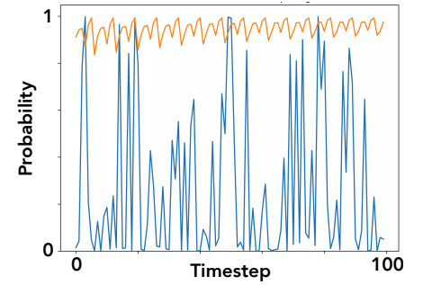
What’s up? Is there a bug? Should we use a bigger beam? Wider, longer? Nope, larger beams don’t help. You can try it for yourself. If you compare human language and machine-generated language, you will see that the conditional probabilities of each subsequent topic are very high for machine-generated texts (beam search is the orange line below) but this is definitely not the case for humans (blue line):
The same effect happens in conversational models. The famous “I don’t know. I don’t know. I don’t know…” answer that plagues many dialogue systems actually has a very high likelihood of occuring, and it gets more probable with each repetition! The loop somehow reinforces itself, and modern attention-based language models easily learn to amplify the bias towards repetition.
On the other hand, humans don’t try to maximize the probability of the next word — that would be very boring! The natural distribution of human texts shown above has a lot of spikes. We are trying to say something, provide information, express emotions.
So what do we do? We can try to sample randomly from the language model distribution. In this case, we begin OK but then quickly degenerate into gibberish. Follow the white rabbit:
This happens because current language models do not work well on the long tail of all words. One uncommon word generated at random from the long tail, and everything breaks down. One way to fix this is to use top-k sampling, i.e., sample randomly but only from the best k options. In our experiments, we no longer get any white rabbits and the text looks coherent enough:
There are still two problems, though. First, there is really no easy way to choose k. The number of truly plausible continuations for a phrase naturally depends on the phrase itself. If k is too large we will get white rabbits, and if k is too small we will get a very bland, boring and possibly repetitive text.
So the next idea is to use top-p sampling, sampling only from the nucleus of the distribution that adds up to a given total probability of say 90% or 95%. In this case, top-p sampling gets some very good results, much more exciting but still coherent enough:
Then Professor Choi talked about GROVER, a recent work from her lab (Rowan Zellers is the first author) that has a huge model with 1.5B parameters able to generate missing variables from the (article, domain, title, author). That is, write an article for a given title, written in the style of a particular author, generate titles from texts, and so on. I won’t go into the details here — GROVER well deserves a separate NeuroNugget, and excellent posts have already been written about it (see, e.g., here). For the purposes of this exposition, let’s just note that GROVER also uses nucleus sampling to generate the wonderful examples that can be found and even generated anew with a demo here.
Nucleus sampling and top-k sampling can also be evaluated in the context of conversational models. Professor Choi actually talked about the Conversation AI 2 challenge, and even made a mistake: she said that the HuggingFace team whose model they used for experiments won the competition, while it was actually us who won (see my earlier post on this). Well, I guess in the large scheme of things it does not matter: our paper at ACL is already a joint effort with HuggingFace, and we hope to keep the collaboration going in the future. As for the comparison, neither top-k nor nucleus sampling was really enough to get an interesting conversation going for a long time.
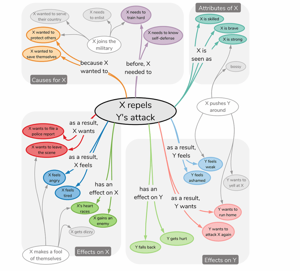
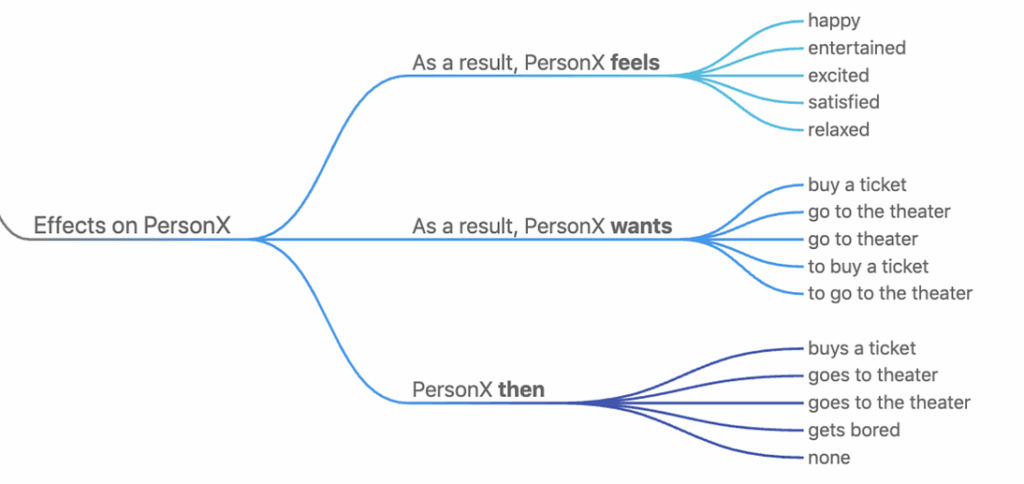
One way to proceed would be to devise models that extract the intent of the speaker from an utterance — finding the reason for the utterance, the desired result, the effect that this might have on the other speakers etc. This work is already underway in Prof. Choi’s lab and they have published a very interesting paper related to it called ATOMIC: An Atlas of Machine Commonsense for If-Then Reasoning. It contains an actual atlas (you could call it a knowledge base) of various causes, effects, and attributes. Here is a tiny subset:
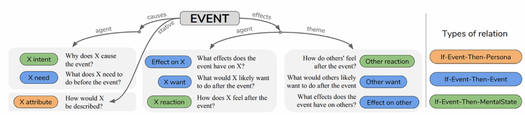
In total, ATOMIC is a graph with nearly 900K commonsense “if-then” rules like the ones above. This is probably the first large-scale effort to collect such information. There are plenty of huge knowledge bases in the world, but they usually contain taxonomic knowledge, knowledge of “what” rather than “why” and “how”, and ATOMIC begins to fill in this gap. It contains the following types of relations:
Building on ATOMIC, Prof. Choi and her lab proceeded to create a model that can construct such commonsense knowledge graphs. This would be, of course, absolutely necessary to achieve true commonsense reasoning: you can’t crowdsource your way through every concept and every possible action in the world.
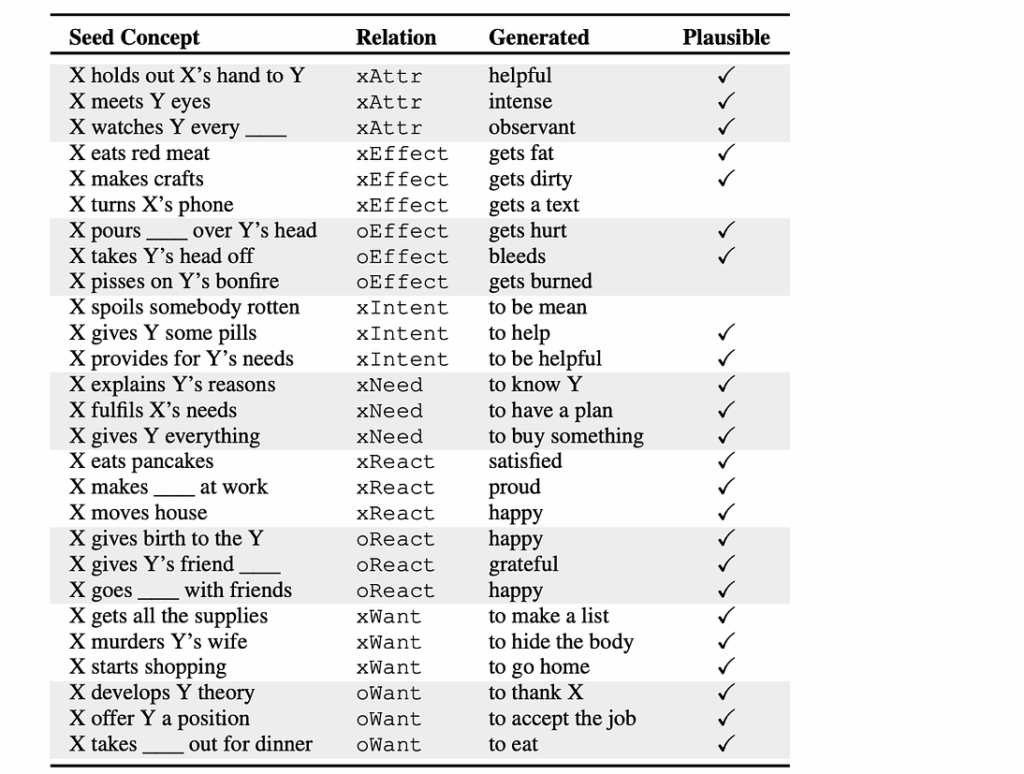
The result is a paper called “COMET: Commonsense Transformers for Automatic Knowledge Graph Construction”. With a Transformer-based architecture, the authors produce a model that can even reason about complex situations. Here is a random sample of COMET’s predictions, with the last column showing human validation of plausibility:
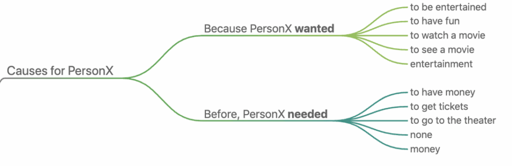
Looks good, right? And here are some predictions for causes and effects for the phrase “Eric wants to see a movie”, answering the question — ‘Why would that be?’
and, ‘What would be the effect if Eric got his wish?’
Models like this suggest that we can try to write down declarative knowledge like this and have a fighting chance of constructing models that, somewhat surprisingly, are able to generalize well to previously unseen events and achieve near-human performance. Will this direction lead to true understanding of the world around us? I cannot be sure, of course, and neither can Professor Choi. But some day, we will succeed in making AI understand. Just you wait.
A Hybrid Model for Globally Coherent Story Generation
And now let us switch to a sample presentation from the Storytelling Workshop. Zhai Fangzhou et al. (ACL Anthology) presented a new model for generating coherent stories based on a given agenda. What does this mean? Natural language generation is basically the procedure of translating semantics into proper language structures, and a neural NLG system will usually consist of a language model and a pipeline that establishes how well and how fully the language structures we generate reflect the semantics, i.e., what we want to say. One example is the Neural Checklist model (Kiddon et al., 2016) where a checklist keeps track of the generation process (have we mentioned this yet?), and another is the Hierarchical seq2seq (Fan et al., 2019, actually presented right here at the ACL 2019).
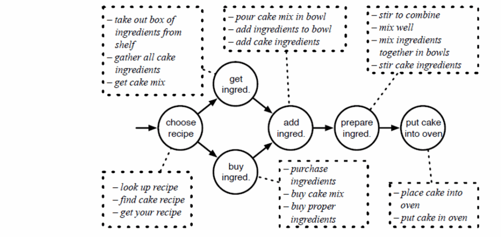
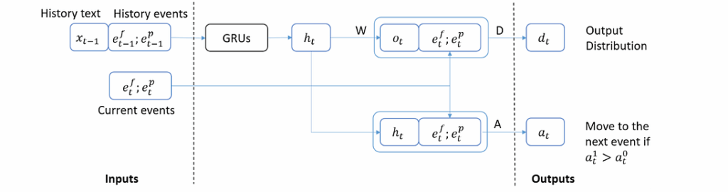
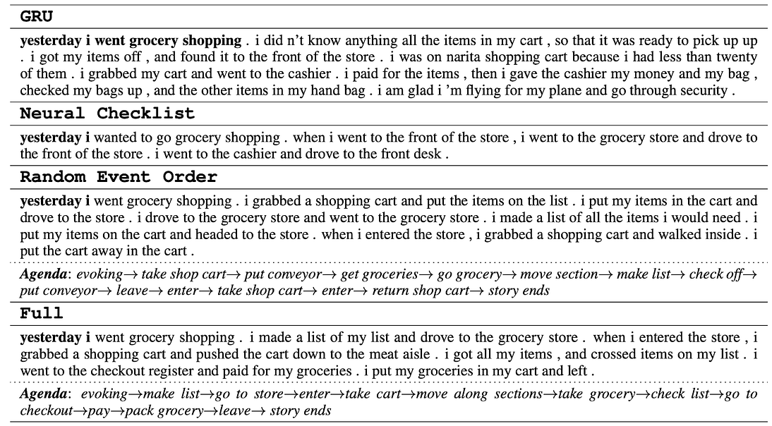
The model by Fangzhou et al. tries to generate coherent stories about daily activities. It has a symbolic text planning component where you write scripts that reflect standardized sequences of events about daily activities. A script is a graph that reflects how the story should progress. It contains events that detail these daily activity scenarios, and the corpus for training contains texts labeled (through crowdsourcing) with these events. Here is a sample data point:
This kind of labeling is hard, so, naturally, the labeled dataset is tiny, about 1000 stories. Another source of data are the temporal script graphs (TSG) that arrange script events according to their temporal and/or causal order. Here is a sample TSG for baking a cake:
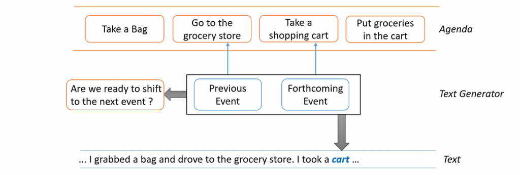
So the proposed model would have an agenda (a sequence of events that plans the story), and the NLG part attends to the most relevant events and decides whether the current event has been annotated and if we can proceed to the next one. In general, it looks like this:
How do you implement all this? Actually, it’s rather straightforward: you use a language model and condition it on the embeddings of currently relevant events. Here is the general scheme:
Let’s see what kind of stories this model can generate. Here is a comparison of several approaches, with the full model in the last place. It is clear that the full model is indeed able to generate the most coherent story that best adheres to the agenda:
These improvements are also reflected in human evaluations: agenda coverage, syntax, and relevance of the full model approach, but still remain below the marks given by human assessors to human-written stories.
In general, this is a typical example of what the Second Storytelling Workshop was about: it looks like good progress is being made, and it seems quite possible to achieve perfection with this kind of story generation quite soon. Add a better language model, label a larger dataset by spending more time and money on crowdsourcing, improve the phrase/event segmentation part, and the result should be virtually indistinguishable from human stories that are similarly constrained on a detailed agenda. But it is clear that this approach can only work in very constrained domains, and what you can actually do with these stories is quite another matter…
Sergey Nikolenko Chief Research Officer, Neuromation
The New Year is here, which means it’s time to relax a little and venture into something interesting, if hypothetical. In this holiday-edition NeuroNugget, we will review the current state of deep learning… but from the point of view of artificial general intelligence (AGI). When are we going to achieve AGI? Is there even any hope? Let’s find out! We begin with a review of how close various fields of deep learning currently are to AGI, starting with computer vision.
Deep Learning: Will the Third Hype-Wave be the Last?
Recently, I’ve been asked to share my thoughts on whether current progress in deep learning can lead to developing artificial general intelligence (AGI), in particular, human-level intelligence, anytime soon. Come on, researchers, when will your thousands of papers finally get us to androids dreaming of electric sheep? And it so happens that also very recently a much more prominent researcher, Francois Chollet, decided to share his thoughts on measuring and possibly achieving general intelligence in a large and very interesting piece, On the Measure of Intelligence. In this new mini-blog-series, I will try to show my vision of this question, give you the gist of Chollet’s view, and in general briefly explain where we came from, what we have now, and whether we are going in the direction of AGI.
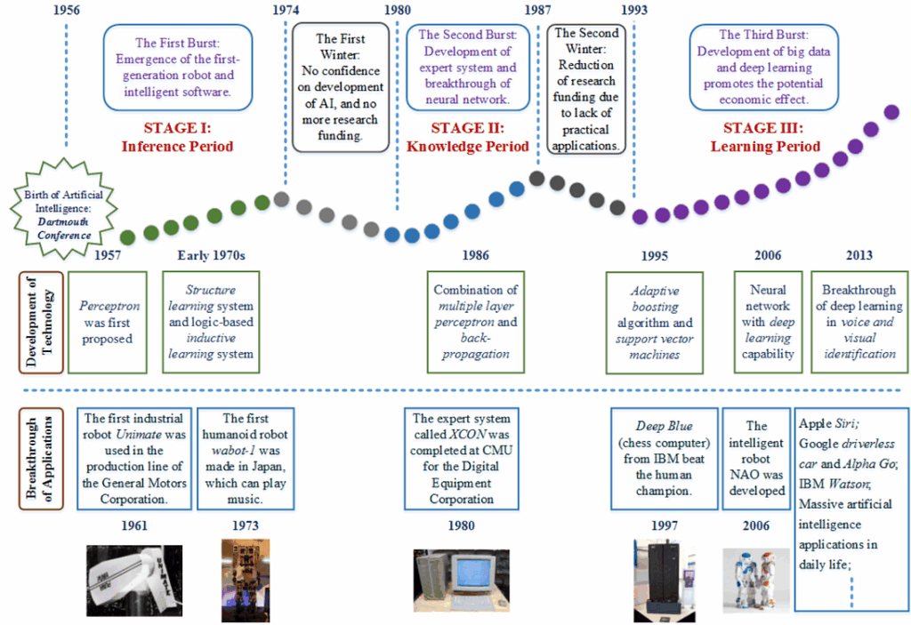
In this blog, we have talked many times about the third “hype-wave” of artificial intelligence that began in 2006–2007, and that encompasses the deep learning revolution that fuels most of the wonderful AI advances we keep hearing about. Deep learning means training AI architectures based on deep neural networks. So the industry has come full circle: artificial neural networks were actually the first AI formalism, developed back in the 1940s when nobody even thought of AI as a research field.
Actually, there have been two full circles because artificial neural networks (ANNs) have fueled both previous “hype waves” for AI. Here is a nice illustration from (Jin et al., 2018):
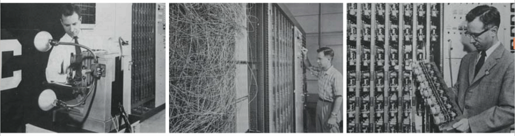
The 1950s and 1960s saw the first ANNs implemented in practice, including the famous Perceptron by Frank Rosenblatt, which was actually a one-neuron neural network, and it was explicitly motivated as such (Dr. Rosenblatt was a neurobiologist and a psychologist, among other things). The second wave came in the second half of the 1980s, and it was mostly caused by the popularization of backpropagation — people suddenly realized they could compute (“propagate”) the gradient of any composition of elementary functions, and it looked like the universal “master algorithm” that would unlock the door to AI. Unfortunately, neither the 1960s nor the 1980s could supply researchers with sufficient computational power and, even more importantly, sufficient data to make deep neural networks work. Here is the Perceptron by Frank Rosenblatt in its full glory; for more details see, e.g., here:
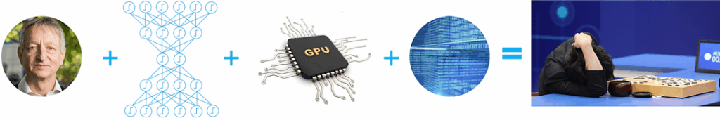
Neural networks did work in the mid-2000s, however. Results coming from the groups of Geoffrey Hinton, Yoshua Bengio, and Yann LeCun — they each had different approaches but were all instrumental for the success of deep learning — made neural networks go from being “the second best way of doing just about anything” (a famous quote from the early 1990s usually attributed to John Denker) to an approach that kept revolutionizing one field of machine learning after another. Deep learning was, in my opinion, as much a technological revolution as a mathematical one, and it was made possible by the large datasets and new computational devices (GPUs, for one) that became available in the mid-2000s. Here is my standard illustration for the deep learning revolution (we’ll talk about the guy on the right later):
It would be impossible to give a full survey of the current state of deep learning in a mere blog post; by now, that would require a rather thick book, and unfortunately this book has not yet been written. But in this first part of our AGI-related discussion, I want to give a brief overview of what neural networks have achieved in some important fields, concentrating on comparisons with human-level results. Are current results paving the road to AGI or just solving minor specific problems with no hope for advanced generalization? Are we maybe even already almost there?
Computer Vision: A Summer Project Gone Wrong
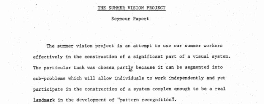
Computer vision is one of the oldest and most important fields of artificial intelligence. As usual in AI, it began with a huge understatement. In 1966, Seymour Papert presented the Summer Vision Project; the idea was to use summer interns in MIT to solve computer vision, that is, solve segmentation and object detection in one fell swoop. I’m exaggerating, but only a little; here is the abstract as shown in the memo (Papert, 1966):
This summer project proved to last for half a century and counting. Even current state of the art systems do not entirely solve such basic high-level computer vision problems as segmentation and object detection, let alone navigation in the 3D world, scene reconstruction, depth estimation and other more ambitious problems. On the other hand, we have made excellent progress, and human vision is also far from perfect, so maybe our current progress is already sufficient to achieve AGI? The answer, as always, is a resounding yes and no, so we need to dig a little deeper.
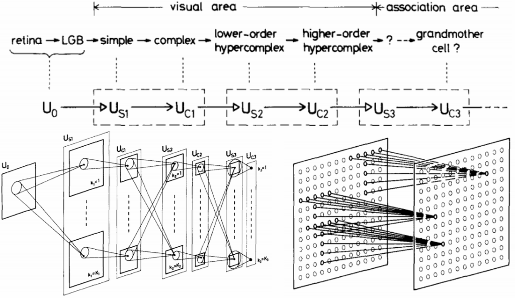
Current state of the art computer vision systems are virtually all based on convolutional neural networks (CNN). The idea of CNNs is very old: it was inspired by the studies of the visual cortex made by Hubel and Wiesel back in the 1950s and 1960s and implemented in AI by Kunihiko Fukushima in the late 1970s (Fukushima, 1980). Fukushima’s paper is extremely modern: it has a deep multilayer architecture, intended to generalize from individual pixels to complex associations, with interleaving convolutional layers and pooling layers (Fukushima had average pooling, max-pooling came a bit later). A few figures from the paper say it all:
Since then, CNNs have been a staple of computer vision; they were basically the only kind of neural networks that continued to produce state of the art results through the 1990s, importantly in LeCun’s group. Still, in the 1990s and 2000s the scale of CNNs that we could realistically train was insufficient to get real breakthroughs.
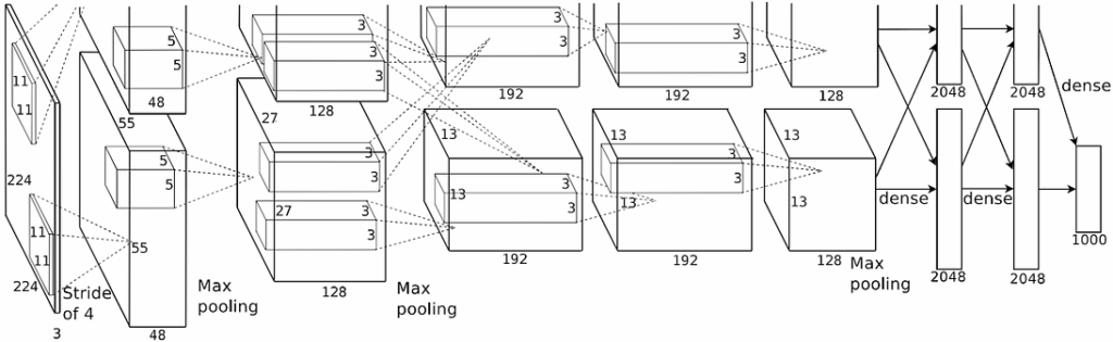
The deep learning revolution came to computer vision in 2010–2011, when researchers learned to train neural networks on GPUs. This significantly expanded the possibilities of deep CNNs, allowing for much deeper networks with much more units. The first problem successfully solved by neural networks was image classification. A deep neural network from Jurgen Schmidhuber’s group (Ciresan et al., 2011) won a number of computer vision competitions in 2011–2012, beating state of the art classical solutions. But the first critically acclaimed network that marked the advent of deep learning in computer vision was AlexNet, coming from Geoffrey Hinton’s group (Krizhevsky et al., 2017), which won the ILSVRC 2012 competition on large-scale image classification based on the ImageNet dataset. It was a large network that fit on two GPUs and took a week to train.
But the results were astonishing: in ILSVRC 2012, the second place was taken by the ISI team from Japan with a classical approach, achieving 26.2% classification error (out of five attempts); AlexNet’s error was 15.3%…
Since then, deep convolutional networks became the main tool of computer vision for practically all tasks: image classification, object detection, segmentation, pose detection, depth estimation, video processing, and so on and so forth. Let us briefly review the main ideas that still contribute to state of the art architectures.
Architectural Ideas of Convolutional Networks
AlexNet (Krizhevsky et al., 2017) was one of the first successful deep CNNs, with more than 20 layers; moreover, AlexNet features model parallelization, working on two GPUs at once:
At the time, it was a striking engineering feat but by now it has become common practice and you can get a distributed model with just a few lines of code in most modern frameworks.
New models appearing in 2013–2015 supplemented the main idea of a deep CNN with new architectural features. The VGG series of networks (Simonyan, Zisserman, 2014) represented convolutions with large receptive fields as compositions of 3х3 convolutions (and later 1xn and nx1 convolutions); this allows us to achieve the same receptive field size with fewer weights, while improving robustness and generalization. Networks from the Inception family (Szegedy et al., 2014) replaced basic convolutions with more complex units; this “network in network” idea is also widely used in modern state of the art architectures.
One of the most influential ideas came with the introduction of residual connections in the ResNet family of networks (He et al., 2015). These “go around” a convolutional layer, replacing a layer that computes some function F(x) with the function F(x)+x:
This was not a new idea; it had been known since the mid-1990s in recurrent neural networks (RNN) under the name of the “constant error carousel”. In RNNs, it is a requirement since RNNs are very deep by definition, with long computational paths that lead to the vanishing gradients problem. In CNNs, however, residual connections led to a “revolution of depth”, allowing training of very deep networks with hundreds of layers. Current architectures, however, rarely have more than about 200 layers. We simply don’t know how to profit from more (and neither does our brain: it is organized in a very complex way but common tasks such as object detection certainly cannot go through more than a dozen layers).
All of these ideas are still used and combined in modern convolutional architectures. Usually, a network for some specific computer vision problem contains some backbone network that uses some or all of the ideas above, such as the Inception Resnet family, and perhaps introduces something new, such as the dense inter-layer connections in SqueezeNet or depthwise separable convolutions in the MobileNet family designed to reduce the memory footprint.
This post does not allow enough space for an in-depth survey of computer vision, so let me just make an example of one specific problem: object detection, i.e., the problem of localizing objects in a picture and then classifying them. There are two main directions here (see also a previous NeuroNugget). In two-stage object detection, first one part of the network generates a proposal (localization) and then another part classifies objects in the proposals (recognition). Here the primary example is the R-CNN family, in particular Faster R-CNN (Ren et al., 2015), Mask R-CNN (He et al., 2018), and current state of the art CBNet (Liu et al., 2019). In one-stage object detection, localization and recognition are done simultaneously; here the most important architectures are the YOLO (Redmon et al., 2015; 2016; 2018) and SSD (Liu et al., 2015) families; again, most of these architectures use some backbone (i.e., VGG or ResNet) for feature extraction and augment it with new components that are responsible for localization. And, of course, there are plenty of interesting ideas, with more coming every week: a recent comprehensive survey of object detection has more than 300 references (Jiao et al., 2019).
No doubt, modern CNNs have made a breakthrough in computer vision. But what about AGI? Are we done with the vision component? Let’s begin with the positive side of the issue.
Superhuman Results in Computer Vision
From the very beginning of the deep learning revolution in computer vision, results have appeared that show deep neural networks outperform people in basic computer vision tasks. Let us briefly review the most widely publicized results, some of which we have actually already discussed.
The very first deep neural net that overtook its classical computer vision predecessors was developed by Dan Ciresan under the supervision of Jurgen Schmidhuber (Ciresan et al., 2011) and was already better than humans! At least it was in some specific, but quite important tasks: in particular, it achieved superhuman performance in the IJCNN Traffic Sign Recognition Competition. The average recognition error of human subjects on this dataset was 1.16%, while Ciresan’s net achieved 0.56% error on the test set.
The main image classification dataset is ImageNet, featuring about 15 million images that come from 22,000 classes. If you think that humans should have 100% success rate on a dataset that was, after all, collected and labeled by humans, think again. During ImageNet collection, the images were validated with a binary question “is this class X?”, quite different from the task “choose X with 5 tries out of 22000 possibilities”. For example, in 2014 a famous deep learning researcher Andrej Karpathy wrote a blog post called “What I learned from competing against a ConvNet on ImageNet”; he spent quite some time and effort and finally evaluated his Top-5 error rate to be about 5% (for a common ImageNet subset with 1,000 classes).
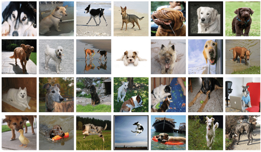
You can try it yourself, classifying the images below (source); and before you confidently label all of them “doggie”, let me share that ImageNet has 120 different dog breeds:
The first network that claimed to achieve superhuman accuracy on this ImageNet-1000 dataset was the above-mentioned ResNet (He et al., 2015). This claim could be challenged, but by now the record Top-5 accuracy for CNN architectures has dropped below 2% (Xie et al., 2019), which is definitely superhuman, so this is another field where we’ve lost to computers.
But maybe classifying dog breeds is not quite what God and Nature had in mind for the human race? There is one class of images that humans, the ultimate social animals, are especially good at recognizing: human faces. Neurobiologists argue that we have special brain structures in place for face recognition; this is evidenced, in particular, by the existence of prosopagnosia, a cognitive disorder in which all visual processing tasks are still solved perfectly well, and the only thing a patient cannot do is recognize faces (even their own!).
So can computers beat us at face recognition? Sure! The DeepFace model from Facebook claimed superhuman face recognition as early as 2014 (Taigman et al., 2014), FaceNet (Schroff et al., 2015) came next with further improvements, and the current record on the standard Labeled Faces in the Wild (LFW) dataset us 99.85% (Yan et al., 2019), while human performance on the same problem is only 97.53%.
Naturally, for more specialized tasks, where humans need special training to perform well at all, the situation is even better for the CNNs. Plenty of papers show superhuman performance on various medical imaging problems; for example, the network from (Christiansen et al., 2018) recognizes cells on microscopic images, estimates their size and status (whether a cell is dead or alive) much better than biologists, achieving, for instance, 98% accuracy on dead/alive classification as compared to 80% achieved by human professionals.
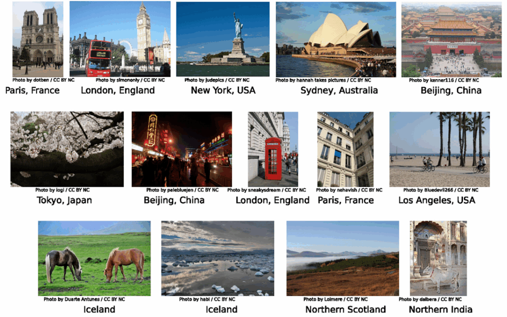
As a completely different sample image-related problem, consider geolocation, i.e., recognizing where a photo was taken based only on the pixels in the photo (no metadata). This requires knowledge of common landmarks, landscapes, flora, and fauna characteristic for various places on Earth. The PlaNet model, developed in Google, already did it better than humans back in 2016 (Weyand et al., 2016); here are some sample photos that the model localizes correctly:
With so many results exceeding human performance, can we say that computer vision is solved by now? Is it a component ready to be plugged into a potential AGI system?
Why Computer Vision Is Not There Yet
Unfortunately, no. One sample problem that to a large extent belongs to the realm of computer vision and has obvious huge economical motivation is autonomous driving. There are plenty of works devoted to this problem (Grigorescu et al., 2019), and there is no shortage of top researchers working on it. But, although, say, semantic segmentation is a classical problem solved quite readily by existing models, there are still no “level 5” autonomous driving models (this is the “fully autonomous driving” level from the Society of Automotive Engineers standard).
What is the problem? One serious obstacle is that the models that successfully recognize two-dimensional images “do not understand” that these images are actually projections of a three-dimensional world. Therefore, the models often learn to actively use local features (roughly speaking, textures of objects), which then hinders generalization. A very difficult open problem, well-known to researchers, is how to “tell” the model about the 3D world around us; this probably should be formalized as a prior distribution, but it is so complex that nobody yet has good ideas on what to do about it.
Naturally, researchers have also developed systems that work with 3D data directly; in particular, many prototypes of self-driving cars have LiDAR components. But here another problem rears its ugly head: lack of data. It is much more difficult and expensive to collect three-dimensional datasets, and there is no 3D ImageNet at present. One promising way to solve this problem is to use synthetic data (which is naturally three-dimensional), but this leads to the synthetic-to-real domain transfer problem, which is also difficult and also yet unsolved (Nikolenko, 2019).
The second problem, probably even more difficult conceptually, is the problem-setting itself. Computer vision problems where CNNs can reach superhuman performance are formulated as problems where models are asked to generalize the training set data to a test set. Usually the data in the test set are of the same nature as the training set, and even models that make sense in the few-shot or one-shot learning setting usually cannot generalize freely to new classes of objects. For example, if a segmentation model for a self-driving car has never seen a human on a Segway in its training set, it will probably recognize the guy as a human but will not be able to create a new class for this case and learn that humans on Segways move much faster than humans on foot, which may prove crucial for the driving agent. It is quite possible (and Chollet argues the same) that this setting represents a conceptually different level of generalization which requires completely novel ideas.
Today, we have considered how close computer vision is to a full-fledged AGI component. Next time, we will continue this discussion and talk about natural language processing: how far are we from passing the Turing Test? There will be exciting computer-generated texts but, alas, much fewer superhuman results there…
Sergey Nikolenko Chief Research Officer, Neuromation
Today, we are still working our way through the ACL 2019 conference. In the fourth part of our ACL in Review series (see the first, second, and third parts), I’m highlighting the “Machine Learning 4” section from the third and final day of the main conference (our final installment will be devoted to the workshops). Again, I will provide ACL Anthology links for the papers, and all images in this post are taken from the corresponding papers unless specified otherwise.
In previous parts, I took one paper from the corresponding section and highlighted it in detail. Today, I think that there is no clear leader among the papers discussed below, so I will devote approximately equal attention to each; I will also do my best to draw some kind of a conclusion for every paper.
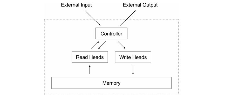
Episodic Memory Reader: Learning What to Remember for Question Answering from Streaming Data
When interacting with a user, a conversational agent has to recall information provided by the user. At the very least, it should remember your name and vital info about you, but actually there is much more context that we reuse through our conversations. How do we make the agent remember?
The simplest solution would be to store all information in memory, but all the context simply would not fit. Moonsu Han et al. (ACL Anthology) propose a model that learns what to remember from streaming data. The model does not have any prior knowledge of what questions will come, so it fills up memory with supporting facts and data points, and when the memory is full, it then has to decide what to delete. That is, it needs to learn the general importance of an instance of data and which data is important at a given time.
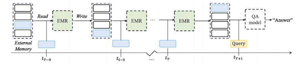
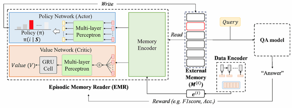
To do that, they propose using the Episodic Memory Reader, a question answering (QA) architecture that can sequentially read input contexts into an external memory, and when the memory is full, it decides what to overwrite there:
To learn what to remember, the model uses reinforcement learning: the RL agent decides what to erase/overwrite, and if the agent has done a good action (discarded irrelevant information and preserved important data), the QA model should reward it and reinforce this behaviour. In total, the EMR has three main parts:
data encoder that encodes input data to the memory vector representation,
memory encoder that computes the replacement probability by considering the importance of memory entries (there are three different variations that the authors consider here), and
value network that estimates the value of the network as a whole (the authors compare A3C and REINFORCE here as RL components).
Here is the general scheme:
To train itself, the model answers the next question with its QA architecture and treats the result (quality metrics for each answer) as a reward for the RL part. I will not go into much formal detail as it is relatively standard stuff here. The authors compared EMR-biGRU and EMR-Transformer (the names are quite self-explanatory: the second part marks the memory encoder architecture) on several question answering datasets, including even TVQA, a video QA dataset. The model provided significant improvements over the previous state of the art.
When I first heard the motivation for this work, I was surprised: how is it ever going to be a problem to fit a dialogue with a human user into memory? Why do we need to discard anything at all? But then the authors talked about video QA, and the problem became clear: if a model is supposed to watch a whole movie and then discuss it, then sure, memory problems can and will arise. In general, this is another interesting study that unites RNNs (and/or self-attention architectures) with reinforcement learning into a single end-to-end framework that can do very cool things.
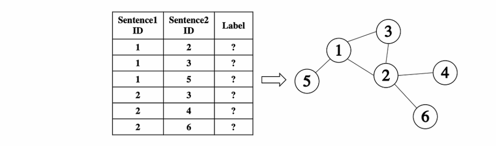
Selection Bias Explorations and Debiasing Methods for Natural Language Sentence Matching Datasets
The second paper presented in the section, by Guanhua Zhang et al. (ACL Anthology), deals with natural language sentence matching (NLSM): predicting the semantic relationship between a pair of sentences, e.g., are they paraphrases of each other and so on.
The genesis of this work was a Quora Question Pairs competition on Kaggle where the problem was to identify duplicate questions on Quora. To find out whether two sentences are paraphrases of each other is a very involved and difficult text understanding problem. However, Kagglers noticed that there are “magic features” that have nothing to do with NLP but can really help you answer whether sentence1 and sentence2 are duplicates. Here are three main such features:
S1_freq is the number of occurrences of sentence1 in the dataset;
S2_freq is the number of occurrences of sentence2 in the dataset;
S1S2_inter is the number of sentences that are compared with both sentence1 and sentence2 in the dataset.
When both S1_freq and S2_freq are large, the sentence pairs tend to be duplicated in the dataset. Why is that? We will discuss that below, but first let’s see how Zhang et al. generalize these leakage features.
The authors consider an NLSM dataset as a graph, where nodes correspond to sentences and edges correspond to comparing relations. Leakage features in this case can be seen as features in the graph; e.g., S1_freq is the degree of the sentence1 node, S2_freq is the degree of the sentence2 node, and S1S2_inter is the number of paths of length 2 between these nodes.
By introducing some more advanced graph-based features that are also kind of “leakage features” and testing classical NLSM datasets for this, the authors obtain amazing results. It turns out that only a few leakage features are sufficient to approach state of the art results in NLSM obtained with recurrent neural models that actually read the sentences!
The authors identify reasons why these features are so important: they are the result of selection bias in dataset preparation. For example, in QuoraQP the original dataset was imbalanced, so the organizers supplemented it with negative examples, and one source of negative examples were pairs of “related questions” that are assumed to be non-equivalent. But a “related question” is unlikely to occur anywhere else in the dataset. Hence the leakage features: if two sentences both appear many times in the dataset they are likely to be duplicates, and if one of them only appears a few times they are likely not to be duplicates.
To test what the actual state-of-the-art models do, Zhang et al. even created a synthetic dataset where the labels are all “duplicate” because the sentences are simply copied for positive examples and show that all neural network models are also biased: they give lower duplication scores to pairs with low values of leakage features even though in all cases the sentences themselves are simply copied — with perfect duplication all around.
So now that we have proven that everything is bleak and worthless, what do we do? Zhang et al. propose a debiasing procedure based on a so-called leakage-neutral distribution where, first, the sampling strategy is independent from the labels, and second, where the sampling strategy features completely control the strategy, i.e., given the features the sampling is independent of the sentences and their labels. In the experimental study, they show that this procedure actually helps to remove bias.
I believe that this work has an important takeaway for all of us, regardless of the field. The takeaway is that we should always be on the lookout for biases in our datasets. It may happen (and actually often does) that researchers compete and compare on a dataset where, it turns out, most of the result has nothing to do with the actual problem the researchers had in mind. Since neural networks are still very much black boxes, this may be hard to detect, so, again, beware. This, by the way, is a field where ML researchers could learn a lot from competitive Kagglers: when your only objective is to win by any means possible, you learn to exploit the leaks and biases in your datasets. A collaboration here would benefit both sides.
Real-Time Open-Domain Question Answering with Dense-Sparse Phrase Index
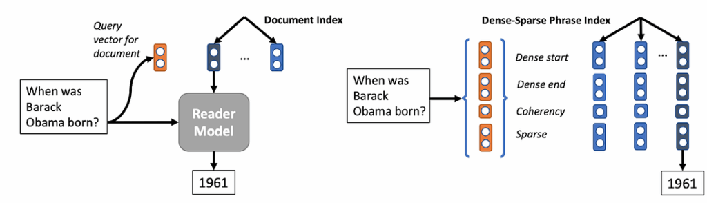
In this work, Minjoon Seo et al. (ACL Anthology) tackle the problem of open-domain question answering (QA). Suppose you want to read a large source of knowledge such as Wikipedia and get a model that can answer general-purpose questions. Real world models usually begin with an information retrieval model that finds the 5–10 most relevant documents and then use a reader model that processes retrieved documents. But this propagates errors from retrieval and is relatively slow. How can we “read” the entire Wikipedia corpus (5 million documents instead of 5–10 documents) and do it quickly (from 30s to under 1s)?
The answer Seo et al. propose is phrase indexing. They build an index of phrase encodings in some vector space (offline, once), and then do nearest neighbor search in this vector space for the query. Here is a comparison, with a standard pipelined QA system on the left and the proposed system on the right:
What do we do for phrase and question representations? Dense representations are good because they can utilize neural networks and capture semantics. But they are not so great at disambiguating similar entities (say, distinguishing “Michelangelo” from “Raphael”), where a sparse one-shot representation would be better. The answer of Seo et al. is to use a dense-sparse representation that combines vectors from a BERT encoding of the phrase and a TF-IDF document and a paragraph unigram and bigram vector in the sparse part.
There are also computational problems. Wikipedia contains about 60 billion phrases: how do you do softmax on 60 billion phrases? Dense representations of 60B phrases would take 240TB of storage, for example. How do you even search in this huge set of dense+sparse representations? So, the authors opted to move to a closed-domain QA dataset, use several tricks to reduce storage space and use a dense-first approach to search. The resulting model fits into a constrained environment (4 P40 GPUs, 128GB RAM, 2TB storage).
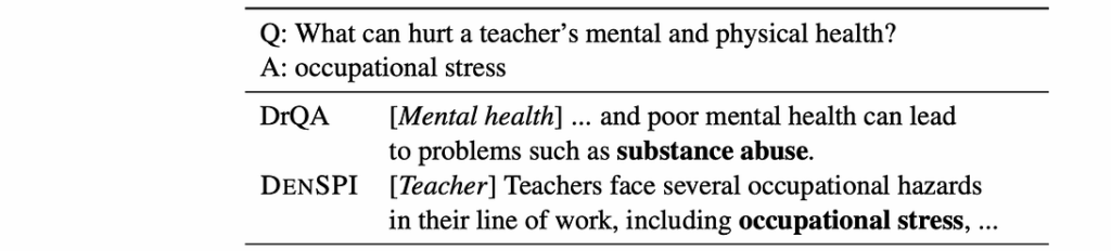
The experimental results are quite convincing. Here are a couple of examples where the previous state of the art DrQA gets the answer wrong, and the proposed DenSPI is right. In the first example, DrQA concentrates on the wrong article:
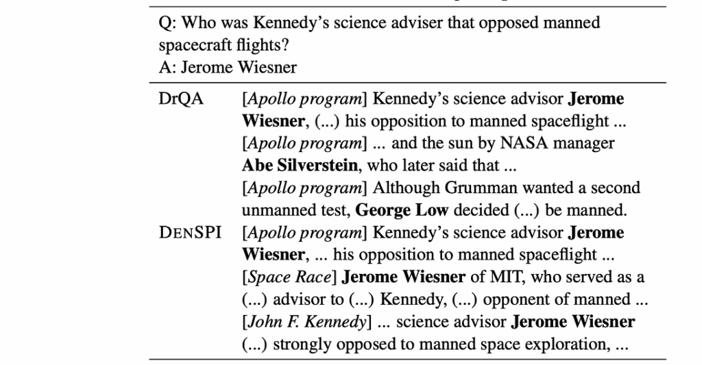
In the second, very characteristic example, DrQA retrieves several answers from a retrieved relevant article and is unable to distinguish between them, while DenSPI can find relevant phrases in other articles as well and thus make sure of the correct answer:
In general, I believe that this approach of query-agnostic indexable phrase representations is very promising and can be applied to other NLP tasks, and maybe even beyond NLP, say in image and video retrieval.
Language Modeling with Shared Grammar
Here we had a hiccup (generally speaking, by the way, ACL 2019 was organized wonderfully: a big thanks goes out to the organizers!): neither of the authors of this paper, Yuyu Zhang and Le Song (ACL Anthology), could deliver a talk at the conference, so we had to watch a video of the talk with slides instead. It was still very interesting.
As we all know, sequential recurrent neural networks are great to generate . But they overlook grammar, which is very important for natural languages and can significantly improve language model performance. Grammar would be very helpful here, but how do we learn it? There are several approaches:
ground truth syntactic annotations can help train involved grammar models but they are very hard to label for new corpora and/or new languages, and they won’t help a language model;
we could train a language model on an available dataset, say Penn Treebank (PTB), and test on a different corpus; but this will significantly reduce the quality of the results;
we could train a language model from scratch on every new corpus, which is very computationally expensive and does not capture the fact that grammar is actually shared between all corpora in a given language.
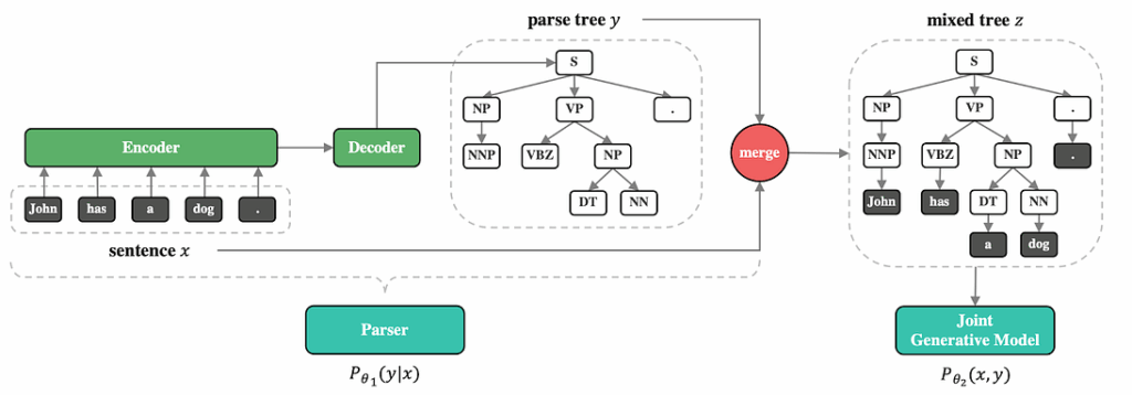
Therefore, Zhang and Song propose a framework for language modeling with shared grammar. Their approach is called the neural variational language model (NVLM), and it consists of two main parts: a constituency parser that produces a parse tree and a joint generative model that generates a sentence from this parse tree.
To make it work, the authors linearize the parse tree with pre-order traversal and parameterize the parser as an encoder-decoder architecture. This set-up allows for several different possible approaches to training:
use a supervised dataset such as PTB to train just the parser part;
distant-supervised learning, where a pre-trained parser is combined with a new corpus without parsing annotations, and we train the joint generative model on the new corpus from generated parse trees (either from scratch or with warm-up on the supervised part);
semi-supervised learning, where after distant-supervised learning the parser and generative models are fine-tuned on the new corpus together, with the variational EM algorithm.
The resulting language model significantly improves perplexity compared with sequential RNN-based language models. I am not sure, however, how this compares with modern state-of-the-art models based on self-attention: can you add grammar to a BERT or GPT-2 model as well? I suppose this is an interesting question for further research.
Densely Connected Graph Convolutional Networks for Graph-to-Sequence Learning
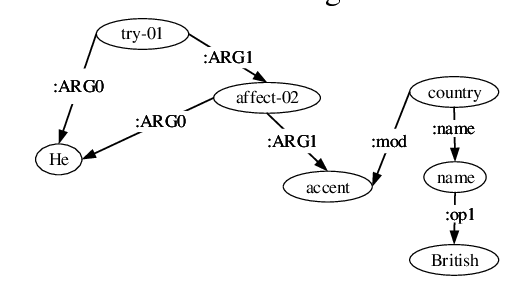
Zhijiang Guo et al. (this is a Transactions of the ACL journal article rather than an ACL conference paper, so it’s not on the ACL Anthology; here is the Singapore University link) consider the problem of graph-to-sequence learning, which in NLP can be represented by, for example, generating text from Abstract Meaning Representation (AMR) graphs; here is a sample AMR graph for the sentence “He tries to affect a British accent”:
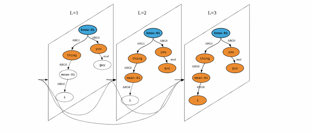
The key problem here is how to encode the graphs. The authors propose to use graph convolutional networks (GCN) that have been successfully used for a number of problems with graph representations. They used deep GCNs to encode AMR graphs, where subsequent layers can capture longer dependencies within the graph, like this:
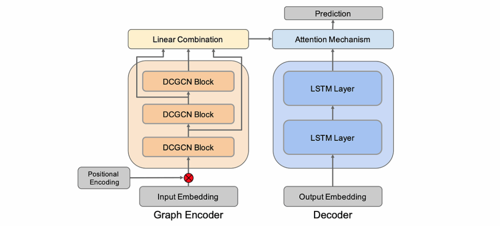
The main part of the paper deals with a novel variation of the graph-to-sequence model that has GCN blocks in the encoder part, recurrent layers in the decoder part, and an attention mechanism controlled by the encoder’s result. Like this:
The authors improve state-of-the-art results on text generation from AMR across a number of different datasets. To be honest, there is not much I can say about this work because I am really, really far from being an expert on AMR graphs. But that’s okay, you can’t expect to understand everything on a large conference like ACL.
This concludes our today’s installment on ACL. That’s almost all, folks; next time I will talk about the interesting stuff that I heard during my last day at the conference at the ACL workshops.
Sergey Nikolenko Chief Research Officer, Neuromation
For the third part of our ACL in Review series, we will be recapping the second day of the ACL 2019 conference (for reference, here are the first part and second part of this series). This section of the conference is titled “Machine Learning 3” and contains several interesting new ideas in different areas of study, three of them united by the common theme of interpretability for models based on deep neural networks and distributed representations. I will provide ACL Anthology links for all papers discussed, and all images in this post are taken from the corresponding papers unless otherwise specified.
For this part, a major recurring theme is interpretability: how do we understand what the model is “thinking”? In NLP, attention-based models have a kind of built-in interpretability in the form of attention weights, but we will see that it is not the end of the story. Also, this time there was no doubt which paper is the highlight of the section: we will see a brand new variation of the Transformer model, Transformer-XL, which can handle much longer context than previous iterations. But we will leave this to the very end, as we are again proceeding in the order in which papers were presented on ACL. Let’s begin!
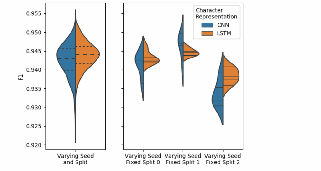
FIESTA: Fast IdEntification of State-of-The-Art models using adaptive bandit algorithms
Throughout machine learning, but especially in NLP, it can be hard to differentiate between the latest models: the results are close, you have to vary both random seeds in the model and train/test splits in the data, and the variance may be quite large. And even after that you still have a very hard decision. Here is a striking real life example from an NLP model with two different character representation approaches:
Which representation should you choose? And how many experiments is it going to take for you to make the correct decision?
To overcome this difficulty, Henry Moore et al. (ACL Anthology) propose to use a well-known technique from the field of reinforcement learning: multi-armed bandits. They are widely used for precisely this task: making noisy comparison choices under uncertainty while wasting as few evaluations as possible. They consider two settings: fixed budget, where you want to make the best possible decision under a given computational budget (given the number of evaluations of various models), and fixed confidence, where you want to achieve a given confidence level for your choices as fast as possible. The authors compare classical algorithms for multi-armed bandits based on Thompson sampling and indeed show that the result becomes better.
To me, using multi-armed bandits for comparison between a pool of models looks like a very natural and straightforward idea that is long overdue to become the industry standard; I hope it will become one in the near future.
Is Attention Interpretable?
Interpretation is an important and difficult problem in deep learning: why did the model make the decision it made? In essence, a neural network is a black box, and any kind of interpretation is often a difficult problem in itself. In this work, Sofia Serrano and Noah A. Smith (ACL Anthology) discuss how to interpret attention in NLP models, where it has been a core mechanism for many recent advances (Transformer, BERT, GPT… more about this below). Attention is very tempting to use as a source of interpretation, as it provides a clear numerical estimate of “how important” a given input is, and this estimate often matches our expectations and intuition. If you look in the papers that use attention-based models, you will often see plots and heatmaps of attention weights that paint a very clear and plausible picture.
But, as the authors show in this work, things are not quite that simple. There are a number of intuitions that may go wrong. For example, we may think that higher-weight representations should be more responsible for the final decision than lower-weight representations. But that’s simply not always true: even the simplest classifier may have different thresholds for different input features. The authors present several tricks designed to overcome this and other similar problems and to test for real interpretability. As a result, they find that attention does not necessarily correspond to importance: even the highest attention weights often do not correspond to the most important sets of inputs, and the set of inputs you have to flip to get a different decision may be too large to be useful for a meaningful interpretation.
The conclusion is unsurprising: with attention, as with mostly everything else, you should proceed with caution. But, to be honest, I don’t really expect this paper to change the way people feel about attention weights: they are still very tempting to interpret, and people still will. A little bit more carefully, maybe.
Correlating Neural and Symbolic Representations of Language
In a way, we continue the theme of interpretability with this paper. How can we understand neural representations of language? One way is to use features such as word embeddings, sentence embeddings, and the like to train diagnostic models, simple classifiers that recognize information of interest (say, parts of speech) and then analyze how these classifiers work. This is well and good when the information of interest is simple, such as a part-of-speech tag, but what if we have a more complex structure such as a parse tree?
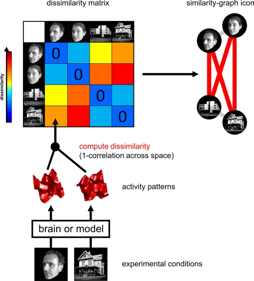
Grzegorz Chrupala and Afra Alishahi (ACL Anthology) present a work where they propose to better understand neural representations of language with the help of Representation Similarity Analysis (RSA) and tree kernels. The idea of RSA is to find correspondences between elements of two different data domains by correlating the similarities between them in these two domains, with no known mapping between the domains. Here is an explanatory illustration from a very cool paper where Kriegeskorte et al. used RSA to find relations between multi-channel measures of neural activity, which is about as unstructured a source of data as you can imagine:
RSA can be applied given a similarity/distance metric within spaces A and B, and when there is no need for a metric between A and B. This makes it suitable for our situation, where A is, e.g., the space of real-valued vectors and B is the set of trees.
To validate this approach, the authors use a simple synthetic language with well-understood syntax and semantics that it is possible to fully learn by an LSTM, namely the language of arithmetic expressions with parentheses. To measure the similarity between trees, they use so-called tree kernels, where similarity is based on the amount of common substructures within the trees. As a result, they get a reasonably well-correlated correspondence between representation spaces and parse trees. In general, it seems that this work brings to NLP and interpretation of neural networks a new tool, RSA, and this tool may prove to be very promising in the future.
Interpretable Neural Predictions with Differentiable Binary Variables
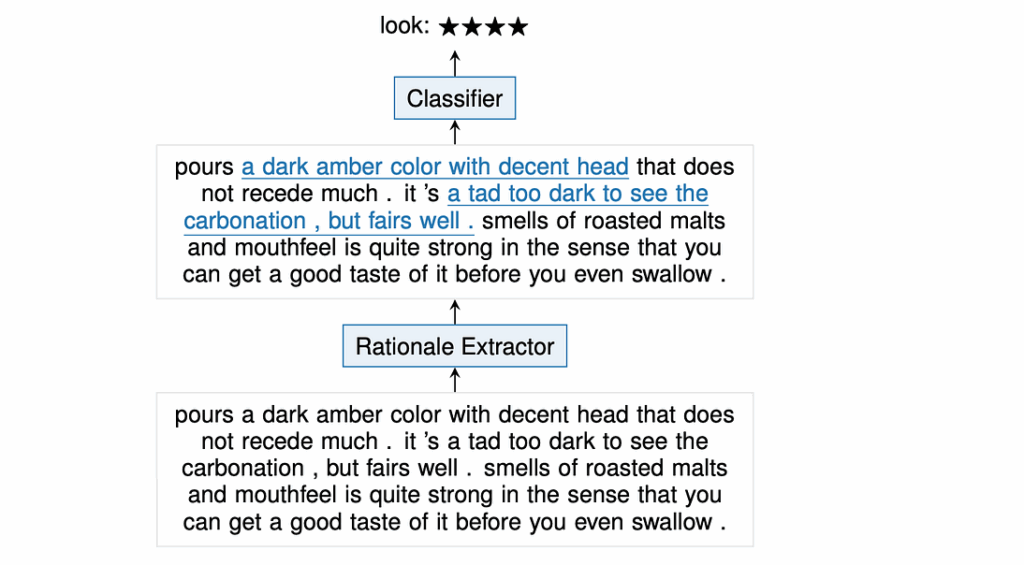
Here again, we continue our investigations into interpretability. Joost Bastings et al. (ACL Anthology) ask the following question: can we make text classifiers more interpretable by asking them to provide a rationale for their decisions? By a rationale they mean highlighting the most relevant parts of the document, a short yet sufficient part that defines the classification result. Here is a sample rationale for a beer review:
Having this rationale, you can, e.g., manually validate the quality of the classifier much faster than you would if you had to read the whole text.
Formally speaking, there is a Bernoulli parameter for every word that corresponds to whether it gets included into the rationale, and the classifier itself works on the masked input after sampling these Bernoulli variables. Sampling is a non-differentiable operation, however, and a classical way to get around this would be to use the reparametrization trick: get samples separately, transform them into Bernoulli variables, and then the gradient can flow through the reparametrization part. To achieve this, the authors use the stretch-and-rectify trick: starting from the Kumaraswamy distribution, which is very similar to the Beta distribution, first stretch it to include 0 and 1 in the support and then rectify by passing it through a hard sigmoid. The transition penalties are still non-differentiable but now admit a Lagrangian relaxation; I will not go into the mathematical details and refer to the paper for all the details.
Suffice it to say, the resulting model does work, can produce rationales for short texts such as reviews with the sentiment classifier on top, and the results look quite interpretable. They also show how to use this as a hard attention mechanism that can replace standard attention in NLP models. This results in a very small drop of accuracy (~1%) but very sparse attention weights (~8.5% nonzero attention weights), which is also very good for interpretability (in particular, most of the critiques from the paper we discussed above do not apply now).
Transformer-XL: Attentive Language Models Beyond a Fixed-Length Context
And finally, the moment we have all been waiting for. In fact, Transformer-XL is old news: it first appeared on arXiv on January 9, 2019; but the submission and review process takes time, so the paper by Zhang Dai et al. (ACL Anthology) is only just appearing as an official ACL publication. Let’s dig into some details.
As is evident from the title, Transformer-XL is a new variation of the Transformer (Vaswani et al., 2017), the self-attention-based model that has (pardon the pun) completely transformed language modeling and NLP in general. Basically, Transformer does language modeling by the usual decomposition of the probability of a sequence into conditional probabilities of the next token given previous ones. The magic happens in how exactly Transformer models these conditional probabilities, but this will remain essentially the same in Transformer-XL so we won’t go into the details now (someday I really have to write a NeuroNugget on Transformer-based models…).
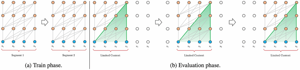
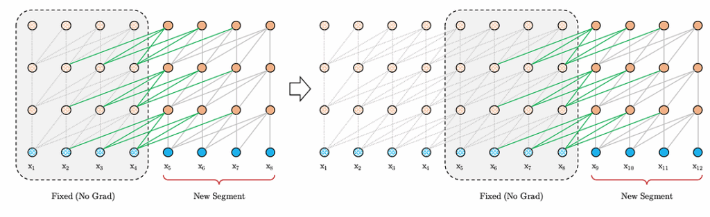
What’s important now is that in the basic Transformer, each token’s attention is restricted so that it does not look “into the future”, and Transformer also reads the segments (say, sentences) one by one with no relation between segments. Like this:
This means that tokens at the beginning of every segment do not have sufficient context, and the entire context is anyway limited to segment length, which is capped at the available memory. Moreover, each new segment requires to recompute the model from the very beginning; basically we start over on every segment.
The key ideas of Transformer-XL designed to solve these problems are:
use segment-level recurrence, where the model caches and reuses hidden states from the last batch; now, each segment can capture the context in the features from previous segments; this extra long context still does not fit into memory, so we cannot propagate gradients back to previous segments, but this is still much better than nothing:
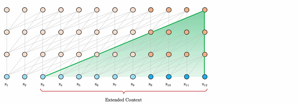
moreover, this idea means that on the evaluation phase, where we do not have to backpropagate the gradients, we are free to use extra-long contexts and do not have to recompute everything from scratch! This speeds things up significantly; here is how it works at the evaluation phase:
There is a new problem now, however. Transformer relies on positional encodings to capture the positions of words in the segment. This stops working in Transformer-XL because now the extra long context relies on words from previous segments, so their positional encodings would be the same, and chaos would ensue.
The solution of Dai et al. is quite interesting: let’s encode distances on edges rather than absolute positions! When the token attends to its immediate predecessor, we add an embedding of distance 0, when it attends to the previous token we add the “distance 1” embedding, and so on.
This allows for much longer contexts, with 4.5x more tokens in the context than the regular Transformer and 80% longer contexts than state of the art RNNs; at the same time, Transformer-XL is up to 1800x (!) times faster than vanilla Transformers. It significantly improves state of the art language modeling results in terms of perplexity, and it is able to generate coherent texts with thousands of tokens.
Finally, let’s see a sample text from the Transformer-XL arXiv paper. First, the seed; Dai et al. initialize Transformer-XL with a long context to provide a lot of information and let it shine by using the whole thing:
= Battle of Dürenstein =
The Battle of Dürenstein (also known as the Battle of <unk>, Battle of <unk> and Battle of <unk>; German: <unk> bei <unk> ), on 11 November 1805 was an engagement in the Napoleonic Wars during the War of the Third Coalition. Dürenstein (modern <unk>) is located in the <unk> Valley, on the River Danube, 73 kilometers (45 mi) upstream from Vienna, Austria. The river makes a crescent-shaped curve between <unk> and nearby Krems an der Donau and the battle was fought in the flood plain between the river and the mountains. At Dürenstein a combined force of Russian and Austrian troops trapped a French division commanded by Théodore Maxime Gazan. The French division was part of the newly created VIII Corps, the so-called Corps Mortier, under command of Édouard Mortier. In pursuing the Austrian retreat from Bavaria, Mortier had over-extended his three divisions along the north bank of the Danube. Mikhail <unk> Kutuzov, commander of the Coalition force, enticed Mortier to send Gazan’s division into a trap and French troops were caught in a valley between two Russian columns. They were rescued by the timely arrival of a second division, under command of Pierre Dupont de l ’Étang. The battle extended well into the night. Both sides claimed victory. The French lost more than a third of their participants, and Gazan’s division experienced over 40 percent losses. The Austrians and Russians also had heavy <unk> to 16 <unk> perhaps the most significant was the death in action of Johann Heinrich von Schmitt, one of Austria’s most capable chiefs of staff. The battle was fought three weeks after the Austrian capitulation at Ulm and three weeks before the Russo-Austrian defeat at the Battle of Austerlitz. After Austerlitz Austria withdrew from the war. The French demanded a high indemnity and Francis II abdicated as Holy Roman Emperor, releasing the German states from their allegiance to the Holy Roman Empire.
= = Background = =
In a series of conflicts from 1803–15 known as the Napoleonic Wars, various European powers formed five coalitions against the First French Empire. Like the wars sparked by the French Revolution (1789 ), these further revolutionized the formation, organization and training of European armies and led to an unprecedented militarization, mainly due to mass conscription. Under the leadership of Napoleon, French power rose quickly as the Grande Armée conquered most of Europe, and collapsed rapidly…
This is a real Wikipedia page, you can check it out here and see how it really continues. But here are the next 1000 tokens generated by Transformer-XL (yes, we do need to have such lengthy examples, the whole point is to see a very long context preserved for a very long time):
after the French conquest of Italy. This victory marked the beginning of the Second Coalition. Napoleon’s rapid advance caused Austria — Russia, Britain and Russia to make peace negotiations. The Russian army under Prince Mikhail Mikhailovich Mikhailovich Chaffee, commander of the Imperial Russian Army in Switzerland, was able to drive off the Austrians in the Battle of Stockach (1805) and to take Pressburg (modern Ö3 Austria) from the Austrians. At an early stage the Austro-Hungarian fleet had been damaged in a storm off Cape Matapan; this allowed the Allies to launch a full-scale invasion of Italy in February 1805. The Battle of Austerlitz was the decisive French victory against Napoleon and the largest naval battle in history, involving more modern-day European navies. The French military situation worsened as Napoleon faced several threats related to his newly formed Army of Europe, particularly Russia itself, which was now on the verge of collapse. The Russian general and friend of Napoleon, Alexander, had been dissatisfied with the conduct of the Austrians; he was still in conflict with Emperor Napoleon, the French Republic’s king, who had declared war on Austria during the summer of 1804. With the war over, Napoleon decided to launch a second invasion of Italy in October 1805.
= = Prelude = =
In July 1805, the French 1st Army entered southern Italy. The army, under the command of Marshal Marmont, were reinforced by a few battalions of infantry under Claude General Auguste de Marmont at the town of Philippsburg and another battalion at Belluno. On 17 September 1805, the army marched from Belluno towards Krems. By 29 September, they had reached Belluno and conducted its advance against a small Austrian force. By 31 September, the whole force had been reinforced by a brigade from the Army of Tyrol under the command of Pierre Augereau. The Austrians were now under the command of Marshal Jean Victor Marie Moreau, a member of the Directory. Moreau had taken command of the Austrian invasion force in the spring of 1805. His command included the VI Corps commanded by Jean Baptiste Drouet de Ney and the VI Corps commanded by Generals Jean Victor Marie Moreau and Joseph Souham. Ney’s corps consisted of the III. Corps and VI. Corps, which consisted of the III Corps and VI. Corps, located in the Austrian Netherlands, was commanded by Friedrich Joseph, Count Baillet de Latour. Moreau’s army consisted of six divisions and several associated brigades.
= = Aftermath = =
= = = First Coalition forces = = =
On 9 October 1805 the French Army of the Danube was attacked by an Austrian army under Archduke Charles at the Battle of Austerlitz. Although Charles and Charles had not had much time to regroup, on 10 October, he launched his attack on the Polish forces under Friedrich Joseph, Count of Lauenburg. After three days, Charles’ army captured Lauenburg. The French forces pursued the Austrians to the Silesian border, where they encountered strong Austrian resistance. These conflicts forced the Austrians to retreat into Tyrol and Austria agreed to a truce. The Austrian army, commanded by Wenzel Anton Karl, Count of Merveldt, was reduced to around 10,000 men. It was initially planned that Archduke Charles would launch a counter-attack against the French army on the same day, as Napoleon had hoped, but this was not carried out. On 25 October, Merveldt left Styria for Tyrol. On the same day, Austria launched its new offensive against the French at Ulm. Charles withdrew his army from the region for a third time at the Battle of Elchingen, under the overall command of the Austrian generals, Ferdinand and Friedrich Wilhelm of Jülich-Cleves-Berg. To prevent Archduke Charles from escaping from the battlefield, the commander of the Habsburg army, Archduke Charles, planned to occupy the fortress Linz; instead, he decided to force Franz von Hipper to surrender the city. However, as Charles moved to the south, Moreau arrived on the scene with additional soldiers — including the entire Imperial Guard — and defeated the Austrians at the Battle of Hohenlinden on 28 October. The loss of Linz resulted in Austria’s complete defeat at Hohenlinden. In the meantime, the French Army of Observation and Preparedness was reorganized into the Army of the Danube under Feldzeugmeister (Colonel-General) Friedrich Freiherr von Hotze. The army was composed of the I, IV, VI, VI, VII, VIII and IX Corps. With reinforcements from Italy and France, it formed new battalions, companies, and squadrons in the Austrian army. On 17 November 1804, at the Battle of Jena-Auerstadt the Army of Silesia and the Army of Silesia joined forces, but by the time that the after the disastrous invasion of Russia in 1812. Napoleon’s empire ultimately suffered complete military defeat in the 1813–14 campaigns, resulting in the restoration of the Bourbon monarchy in France. Although Napoleon made a spectacular return in 1815, known as the Hundred Days, his defeat at the Battle of Waterloo, the pursuit of his army and himself, his abdication and banishment to the Island of Saint Helena concluded the Napoleonic Wars.
= = Danube campaign = =
From 1803–06 the Third Coalition fought the First French Empire and its client states (see table at right ). Although several naval battles determined control of the seas, the outcome of the war was decided on the continent, predominantly in two major land operations in the Danube valley: the Ulm campaign in the upper Danube and the Vienna campaign, in the middle Danube valley. Political conflicts in Vienna delayed Austria’s entry into the Third Coalition until 1805. After hostilities of the War of the Second Coalition ended in 1801, Archduke <unk> emperor’s <unk> advantage of the subsequent years of peace to develop a military restructuring plan. He carefully put this plan into effect beginning in 1803–04, but implementation was incomplete in 1805 when Karl Mack, Lieutenant Field Marshal and Quartermaster-General of the Army, implemented his own restructuring. Mack bypassed Charles ’ methodical approach. Occurring in the field, Mack’s plan also undermined the overall command and organizational structure. Regardless, Mack sent an enthusiastic report to Vienna on the military’s readiness. Furthermore, after misreading Napoleon’s maneuvers in Württemberg, Mack also reported to Vienna on the weakness of French dispositions. His reports convinced the war party advising the emperor, Francis II, to enter the conflict against France, despite Charles ’ own advice to the contrary. Responding to the report and rampant anti-French fever in Vienna, Francis dismissed Charles from his post as generalissimo and appointed his <unk> brother-in-law, Archduke Ferdinand, as commander. The inexperienced Ferdinand was a poor choice of replacement for the capable Charles, having neither maturity nor aptitude for the assignment. Although Ferdinand retained nominal command, day-to-day decisions were placed in the hands of Mack, equally ill-suited for such an important assignment. When Mack was wounded early in the campaign, he was unable to take full charge of the army. Consequently, command further devolved to Lieutenant Field Marshal Karl Philipp, Prince of Schwarzenberg, an able cavalry officer but inexperienced in the command of such a large army.
= = = Road to Ulm = = =
The campaign in the upper Danube valley began in October, with several clashes in Swabia. Near the Bavarian town of Wertingen, 40 kilometers (25 mi) northwest of Augsburg, on 8 October the 1st Regiment of dragoons, part of Murat’s Reserve Cavalry Corps, and grenadiers of Lannes ’ V Corps surprised an Austrian force half its size. The Austrians were arrayed in a line and unable to form their defensive squares quickly enough to protect themselves from the 4,000 dragoons and 8,000 grenadiers. Nearly 3,000 Austrians were captured and over 400 were killed or wounded. A day later, at another small town, <unk> south of the Danube <unk> French 59th Regiment of the Line stormed a bridge over the Danube and, humiliatingly, chased two large Austrian columns toward Ulm. The campaign was not entirely bad news for Vienna. At Haslach, Johann von Klenau arranged his 25,000 infantry and cavalry in a prime defensive position and, on 11 October, the overly confident General of Division Pierre Dupont de l’Étang attacked Klenau’s force with fewer than 8,000 men. The French lost 1,500 men killed and wounded. Aside from taking the Imperial Eagles and <unk> of the 15th and 17th Dragoons, Klenau’s force also captured 900 men, 11 guns and 18 ammunition wagons. Klenau’s victory was a singular success. On 14 October Mack sent two columns out of Ulm in preparation for a breakout to the north: one under Johann Sigismund Riesch headed toward Elchingen to secure the bridge there, and the other under Franz von Werneck went north with most of the heavy artillery. Recognizing the opportunity, Marshal Michel Ney hurried the rest of his VI Corps forward to re-establish contact with Dupont, who was still north of the Danube. In a two-pronged attack Ney sent one division to the south of Elchingen on the right bank of the Danube. This division began the assault at Elchingen. At the same time another division crossed the river to the east and moved west against Riesch’s position. After clearing Austrian pickets from a bridge, the French attacked and captured a strategically located abbey at French approached Vienna, the Prussians had already surrendered. As the Austrians did not want to allow the war to continue, they decided to abandon their territories in the north and move their army to the north and west, cutting off Charles from Vienna. The Battle of Warsaw was fought on 23 November 1805 between the French Army of the Danube and the Austrian Army of Styria in the vicinity of Warsaw and Pressburg (modern Trnava, Slovakia). At that time Habsburg forces…
Transformer-XL is one of the newest state of the art language models, with an attention-based architecture that improves over but also closely follows the original Transformer. This line of models (also including BERT, GPT, and GPT-2) has resulted in unprecedented text generation quality (check out GROVER!), but it’s still clear that there is no true “understanding”, whatever that means. To have that, we need to imbue our models with common sense, that is, some kind of understanding of the world around us. I’ve seen some very smart people at ACL 2019 say that they are working on this problem exactly. Let’s hope they succeed, and see you next time for our next installment!
Sergey Nikolenko Chief Research Officer, Neuromation
Neuromation researchers attended ACL 2019, the Annual Meeting of the Association for Computing Linguistics, which is the world’s leading conference in the field of natural language processing. With this second part of our ACL in Review series (see the first part here), I continue the experiment of writing draft notes as the ACL sections progress.
This time, it’s the Monday evening session called “Vision, Robotics, Multimodal, Grounding and Speech”; this means that in this section, we get some nice pictures along with the text. Again, I will provide ACL Anthology links for the papers, and all images in this post are taken from the corresponding papers unless specified otherwise. The paper I want to discuss in detail was not the first in its section, but I still decided to keep the order from the conference to make it as authentic as possible.
On to the papers!
Visually Grounded Neural Syntax Acquisition
How do we understand syntax? When we were children, we had to derive it from data, from the language stream directed at us. But what really helped was that language was often paired with imagery: by hearing sentences like “A cat is sleeping outside”, “A cat is staring at you”, or “There’s a cat playing with the ball” and matching them with what we saw, we could extract the notion of “a cat”.
Haoyue Shi et al. (ACL Anthology) ask how to implement this technique for deep learning models: can we generate a linguistically plausible structure for the text given a set of parallel image-text data (say, the MS COCO dataset)? They use the notion of “concreteness”: concrete spans in the parse tree such as “a cat” are more likely to correspond to objects on a picture. This notion can be captured by a part of the network that estimates concreteness based on the interrelation between captions and images. The entire network learns a joint embedding space that unites images and constituents in the same vector space with a hinge-based triplet loss; abstractness and concreteness are defined in the same embedding space. In general, the structure looks like this:
With this approach, the authors get a model that jointly learns parse trees and visually grounded textual representations. They show state of the art parsing results with much less data than needed for state of the art text-only models.
Stay on the Path: Instruction Fidelity in Vision-and-Language Navigation
This work by Google researchers Vihan Jain et al. (ACL Anthology) deals with a rapidly growing field of vision-and-language navigation (VLN): how can we give instructions to agents in natural language and have the agents plan their actions, navigate and respond to the changes in their visual field? A characteristic example here would be the Room-to-Room (R2R) dataset that contains images of real indoor environments, where the agent is asked to follow instructions such as, e.g., “Make a left down at the narrow hall beside the office and walk straight to the exit door. Go out the door and wait.” On a map this might look something like this:
The authors move from R2R to R4R, where instructions are more detailed, the paths are longer, and the agent is supposed to follow specific navigation instructions rather than just find the shortest path from point to point. For instance, the agent that found the red path in the right part of the image above would be penalized if the actual instruction was to go along the blue path; the agent using the orange path in the image does a better job even though it fails to actually reach the target.
The models, all based on the reinforced cross-modal matching (RCM) model by Wang et al., now also come in two variations with different rewards: goal-oriented agents just want to reach the goal, while fidelity-oriented agents have an objective function that rewards following the reference path. It is no wonder that the latter does a better job with R4R. Generally, the work argues that path fidelity is a better objective if our goal is to better understand natural language instructions — the problem being to understand the instruction in its entirety rather than just extract the endpoint.
Expressing Visual Relationships via Language
And here comes our highlight for the section on visually grounded NLP. In this work, Adobe researchers Hao Tan et al. (ACL Anthology) move from the already classic problem of imagecaptioning, i.e., describing with natural language what an image contains, to image editing, i.e., describing what we want to do with the image. We want a model that can get a request such as “Add a sword and a cloak to the squirrel” and do something like this:
So the first question is how you collect a dataset of this kind. The supervised dataset should consist of triples: the original image, an editing request, and the modified image. First, the authors crawled a collaborative image editing community called Zhopped (note: I will be hugely surprised if there are no Russian speakers behind this website) and Reddit; specifically, there is a reddit called r/PhotoshopRequest where you can ask people to help you with image editing. This yielded the pairs of original and edited images. Although Reddit and Zhopped both contain the original editing requests from users, these are usually very noisy and often conversational, so the authors opted to re-do all the requests manually through crowdsourcing.
This procedure yielded the image editing dataset. The authors also used the Spot-the-Diff dataset from (Jhamtani, Berg-Kirkpatrick, 2018) that focuses on finding changes between two images. The problem is now to generate text from a pair of images, like this:
The third dataset with image-image-text triples is the NLVR2 dataset (Suhr et al., 2018) that emphasizes the relationship between the two images. Given two images and a statement, you are supposed to classify whether the statement is true or false; for the purposes of this paper, the authors simply used the correct statements and converted this into a captioning problem for a pair of images:
Now that we have the data, what about the models? To be clear, let’s concentrate on the task of generating a sentence that describes the relationship between a pair of images. There are four different models used in the paper, with a natural succession between them. Let’s look at the flowchart and then discuss it:
This is quite a lot to parse, but actually this is a careful build-up of well-known ideas in the field. The first model (a) is an adaptation of the encoder-decoder model with attention, very similar to the ones used by Xu et al. and Jhamtani and Berg-Kirkpatrick. It constructs features from input images, concatenates them, and then uses this as context to predict the next word with a recurrent architecture.
The basic model, however, does not even differentiate between the two input images. To fix this, model (b) moves on to multi-head attention, an idea made very popular in NLP by Transformer and its follow-up models. In model (b), attention is applied sequentially, so that when the model is attending to the target image it can have context from the source image already available, and it can immediately know where to look for differences.
Naturally, this progression means that quality metrics improve as we move from model (a) to model (d). Here are some sample results from the paper, both positive and negative:
As you can see, sometimes state-of-the-art models are actually pretty good at understanding what is going on with the images, but sometimes they are lost and definitely don’t understand what they’re talking about.
Weakly-Supervised Spatio-Temporally Grounding Natural Sentence in Video
Traditional video grounding is the problem of localizing a spatial region in certain video frames that corresponds to a specific part of a natural language query (say, find the part of the “spatio-temporal tube”, i.e., the video tensor, that corresponds to a coffee cup). This, however, requires dense fine-grained regional annotations in the video, which are very hard to obtain, so this work by Zhenfang Chen et al. (ACL Anthology) considers weakly supervised video grounding. Moreover, they move to the general problem of localizing a spatio-temporal tube that corresponds to a given sentence as a whole, not to a specific noun. They call this problem weakly-supervised spatio-temporally grounding sentence in video (WSSTG); like this:
To solve the problem, the authors use a pipeline with a standard Faster R-CNN object detector to generate bounding box proposals (Instance Generator below), an “Attentive Interactor” module that unites RNN-produced representations for the text and the proposed regions, and then the whole thing is trained with a ranking loss and a diversity loss with multiple instance learning. Here is the whole pipeline:
The authors also collect and present a new dataset designed for this problem, with videos where some target regions are annotated with sentences. There is nothing too sensational in this approach, but, as often happens with modern deep learning models, it is a big surprise that it actually does work! The resulting model can correctly understand quite complicated queries. Here is a sample comparison from the paper:
The PhotoBook Dataset: Building Common Ground through Visually-Grounded Dialogue
And the last paper of the day was by Janosch Haber et al. (ACL Anthology). This dataset concentrates not on captioning, but on visually-grounded dialogue, i.e. conversations . The authors argue that one important reason why dialogue is hard is because the participants rely on their shared knowledge and shared linguistic experience that they build during the conversation, and current dialogue models still cannot really capture this “common ground”. So their proposal is to create a dataset where the grounding is not only conversational but also visual. This is implemented as a game: two participants see six photos each, and they need to find out in dialogue which of the three highlighted photos they have in common (some of them are the same and some are different). They do it in natural dialogue, and the visual domain is controlled too, so the images are sufficiently similar to require an in-depth description from the participants. Here is an example:
Moreover, the game consists of five rounds (hence the “Page 1 of 5” in top left), and in subsequent rounds some images can reappear again, which motivates the participants to make mutually referring descriptions of images. Therefore, this large-scale crowdsourced data collection allows the authors to not only have a good dataset for training but also make some conclusions on how people talk about images. Especially interesting conclusions deal with how the game changes over the five rounds: as the game progresses, utterances become much shorter, the fraction of nouns and content words increases significantly, but these words also begin to repeat themselves a lot, so there are fewer new nouns introduced in later rounds. This is exactly the “common ground” that is hard to capture for the conversational model.
Then the authors present two baseline models for visual grounding, one that has no dialogue history and one that receives (in processed form) the references from previous rounds of the conversation. Naturally, the latter model is more successful on later stages of the game; in the example below, both models do just fine in the left example but only the history-based model can manage the example on the right (and no wonder!):
But both models are still far from perfect, and, of course, the authors hope that this dataset will serve as a common ground (pardon the pun) for further research in the field.
With this, we finish the “Vision, Robotics, Multimodal, Grounding and Speech” section. We are often bombarded by stories about sensational AI achievements from the media. Usually the journalists are not trying to lie to us, but it’s often hard to say whether they are showing a best-case cherry-picked example or a solution ready to go to production. Thus, it was very enlightening to see what exactly the state of the art really is in these things. For most models that we’ve seen today, my conclusion is: sometimes they work, and you can find really cool examples if you look, but very often they still get lost. On the other hand, a lot of this research sounds very promising for real world applications as well. We should stay tuned to this research, but it’s clear that true deep understanding of images from the real world and a genuine ability to put images into words or vice versa are still quite far away.
Sergey Nikolenko Chief Research Officer, Neuromation
Neuromation researchers are currently attending ACL 2019, the Annual Meeting of the Association for Computing Linguistics, which is the world’s leading conference in the field of natural language processing. While we do have a paper here, “Large-Scale Transfer Learning for Natural Language Generation”, in this series we will be concentrating on some of the most interesting works we are seeing from others.
Since I am now attending this multi-day conference in person, I’d like to switch gears in my reviews a little. This time, let’s follow the conference as we experience it. Research conferences are usually organized into tracks: you go to a specific room where you listen to several talks united by some common topic. Thus, I will organize this “ACL in Review” NeuroNugget series into ACL tracks that I personally visited. I typed in the rough notes for this piece as I was sitting in on the talks at ACL and later just edited them lightly for readability. For every track, I will choose one paper to highlight in detail and provide very brief summaries of the rest.
So, without further ado, let’s get started! Following is part 1 of my personal experience of the ACL 2019 Conference.
The first track I visited was called “Machine Learning 1”, which was chaired by Chris Dyer, a researcher at DeepMind who is famous for his work in deep learning for NLP. The track collected papers that have ideas of interest for natural language processing and even beyond to machine learning in general. I will begin with the highlight paper and then proceed to describe the rest.
In line with other top NLP conferences, ACL has the laudable tradition of publishing all accepted papers online in the ACL Anthology. So, I will provide ACL Anthology links for the papers we discuss here, rather than arXiv or some other repository. All pictures are taken from the corresponding papers unless specified otherwise.
Augmenting Neural Networks with First Order Logic
As we know, neural networks are great but still suffer from a number of issues. First of all, they are basically end-to-end non-differentiable black boxes, and although they have a lot of hidden variables, these variables are hard to interpret and match with something that we could add external knowledge to. In this work, Tao Li and Vivek Srikumar (ACL Anthology) present a framework for adding domain knowledge to neural networks.
Consider this reading comprehension question answering example from the paper:
In this example, an attention-based model will try to learn an alignment between words in the question and in the paragraph. If you have a huge dataset and a large model, then, of course, mapping “author” to “writing” can occur naturally. If not, however, it is much easier if the network has some way to, e.g., align words that are labelled as similar in some knowledge base. Such knowledge bases, of course, exist and are readily available for most languages.
This is an example where we have domain knowledge about the problem in the form of rules: if the two words are considered related (a binary predicate holds) then align them. There are a lot of things you can encode with such rules if you allow the rules to be expressed in first-order logic, i.e., in the form of logical formulas that can contain predefined predicates. This way to define the rules is very expressible, easy for experts to state and for non-experts to understand, so it is a very natural idea to try to add them to neural networks.
First idea: let’s have named neurons! That is, suppose that some neurons in the networks are associated with an externally-defined meaning. That is, you have a neuron, say a, and another neuron, say b, and you want the result on the next layer, a neuron c, to be a logical conjunction of these two: c=a&b. Sounds like a very easy function to add to the computational graph… but it’s definitely not a differentiable function! Backpropagation will break on a logical “AND” as much as it would break on, say, the argmax function. So how can we insert the predicates and first-order rules into a neural network, where differentiability is paramount?
We need to soften the logical operations, replacing them with differentiable functions in such a way that the result reflects how much we believe the predicate to be true. Li and Srikumar propose to do this with distance functions: given a neuron y=g(Wx) for some activation function g, inputs x, and weights W, and assuming we want to express some conditional statement Z→Y, where Z is some formula over variables z and Y is the variable associated with y, we define a constrained neural layer as y=g(Wx+⍴d(z)), where d(z) is the distance function corresponding to the statement. The authors introduce such functions based on the Lukasiewicz t-norm; say, (NOT a) corresponds to (1-a) and (a&b) corresponds to max(0,a+b-1). Then, provided that your logical formulas do not introduce cycles in the computational graph, you can map them inside the neural network.
The authors augmented several models in this way: a decomposable attention model (Parikh et al., 2016) for natural language inference, BiDAF (Seo et al., 2016) for machine comprehension, and others. For example, in BiDAF the model contains encoded representations of paragraph and query, attention vectors, and the outputs. The logical rules go like this: if two words in the paragraph and query, p and q, are related in the ConceptNet knowledge base, Related(p, q), then align them in the attention layer. As for natural language inference, here the rule is that if Related(p, h) and the unconstrained network strongly believes that the words should align, then align them.
The authors show that the results improve across all experiments, but especially significant improvements result when you have relatively little data: the authors experimented by taking only 1%, 5%, 10% and so on of the same dataset for training. When using 100% of the dataset, there is even a slight deterioration in the results in the case of natural language inference, which probably means that the rules are a little noisy, and the network is already better off learning the rules from data.
Thus, the conclusion is simple: if you have a huge dataset, just believe the data. If not, you may be better off adding external domain knowledge, and this paper gives you one way to add it to our beloved neural black boxes. I hope to see more of this connection between domain knowledge and neural networks in the future: it has always sounded absurd to me to just throw away all the knowledge we have accumulated (although sometimes, like in chess, this is exactly the way to go… oh well, nobody said it would be easy).
This work by Julia Kreutzer and Stefan Riezler (ACL Anthology) presents an interesting way to combine various different supervision types. As you know, machine learning techniques are distinguished by supervision types: supervised, semi-supervised, unsupervised, reinforcement. This work tries to find the right balance between different supervision types and to teach a model to integrate multiple different types of supervision. For example, for sequence-to-sequence learning in machine translation, suppose you have a human “teacher” who can mark and/or correct wrong parts of a translated sentence. The solution is a self-regulation approach based on reinforcement learning: there is a regulator model that chooses the supervision type, which serves as the action for the RL agent. The authors successfully evaluated this approach on the personalization task (online domain adaptation from news to TED talks and from English to German) and on machine translation, where the supervision was simulated with reference translations. This looks a lot like active learning, so they also compared it (favorably) with traditional uncertainty-based active learning techniques.
Neural Sequence-to-Sequence Models from Weak Feedback with Bipolar Ramp Loss
In this work, Laura Jehl et al. (ACL Anthology) consider the often-encountered case when golden ground truth supervision is not available but there is still some weak supervision. For example, in semantic parsing for question answering, it’s much easier to collect question-answer pairs than question-parse pairs. Usually, people solve this problem by using metric-augmented objectives where the external metric can be computed with the “golden” target and can help guide the learning process, but where the metric is removed from the actual structure produced by the model and may be unreliable. The intuition is to use this metric to both reward “good” structures and punish “bad” structures according to this weak feedback.
The authors consider several different objectives: in minimum risk training (MRT), the external metric assigns rewards to model outputs. In the ramp loss objective, the function encourages answers that have high probability and a high feedback score (hope outputs) and discourages answers that have a low feedback score but still a high probability of appearing (fear outputs). In the new objective presented in this work, token-level ramp loss, the ramp loss idea is pushed down to individual tokens, encouraging tokens that occur only in the positive example, discouraging tokens from the negative example, and leaving untouched the tokens that appear in both.
The authors apply these objectives to an encoder-decoder model with attention pretrained with maximum likelihood estimation and report improvements for semantic parsing and weakly supervised machine translation for ramp loss over MRT and for token-level ramp loss over the regular ramp loss.
You Only Need Attention to Traverse Trees
Models based on self-attention have completely transformed the field of natural language processing over the last year. Transformer, BERT, OpenAI GPT and their successors have been instrumental in most of the recent famous NLP advances. In this work (ACL Anthology), Mahtab Ahmed et al. present an extension of the self-attention framework that worked so well for sequences to trees, proposing a Tree Transformer model that can handle phrase-level syntax from constituency trees. Basically, they use the attention module as the composition function in a recursive tree-based structure. I won’t go into much detail but here is their main illustration:
They evaluated their results on the Stanford Sentiment Treebank for sentiment analysis, the Sentences Involving Compositional Knowledge (SICK) dataset for semantic relatedness, and other tasks, getting results close to state of the art tree-structured models and significantly better than the regular Transformer.
The Referential Reader: A Recurrent Entity Network for Anaphora Resolution
In this work from Facebook Research, Fei Liu et al. (ACL Anthology) tackle the hard and interesting problem of anaphora resolution, that is, which concept or previously mentioned word/phrase does a given pronoun refer to? It (please resolve my anaphora here) is an interesting problem, and actually even the very best models are still far from perfect at this task — getting anaphora resolution right in corner cases would require some deep knowledge about the world. The authors present the so-called Referential Reader model: it identifies entity references and stores them in a fixed-length memory, with the update and overwrite operations for the memory available for the model. The memory is controlled with a GRU-based language model, with special saliency weights showing which memory cells are still important and which are safe to overwrite. So, in the example below, we first store the “Ismael” in the first cell and increase its saliency, then overwrite the second cell (with low saliency) with “Captain Ahab” (first “captain”, then updated with “Ahab”), and then resolve the “he” reference by choosing the first memory cell contents:
All of this is controlled with recurrent neural nets (I won’t go into the details of the control mechanism, check the paper for that), and the results significantly improve over current state of the art. Moreover, this approach can benefit from unsupervised pre-training via better language models, and the best results are achieved with state of the art BERT language models.
Adaptive Attention Span in Transformers
And now back to Transformers. The original Transformer is based on a multi-head attention system where each head receives query-key-value triples produced from the input vectors and then combines them into attention values. Sainbayar Sukhbaatar et al. (ACL Anthology) attempt to make self-attention more efficient. The problem they are trying to fix is that networks based on self-attention take into account a very long context (up to 3800 tokens for Transformer-XL), which leads to very high memory requirements for the models since you need to compute self-attention with every context word in every attention head. The authors note that some heads do use the long context (it has been shown that long context in general provides a lot of benefits here) but some do not, using much shorter “attention spans” of only a few tokens. Therefore, the authors introduce adaptive attention spans, adding a special masking function to limit the context length and learning its parameters, thus forcing the model to use shorter spans with special regularization.
The authors compare their models with regular Transformer-based networks and show that they can achieve the same or even slightly better results on held-out test sets with significantly smaller models. Another interesting observation is that in the resulting models, the early layers almost universally use very short attention spans, and only the later layers (say, layers 8–12 in a 12-layer model) can make good use of long contexts. Here are two examples: on the left, we see head B in a regular Transformer caring about much shorter context than head A; on the right, we see the actual attention spans across various layers:
With this, the first track was over; all of these papers were presented as 15–20 min talks, with less than two hours for all of the above, including questions and technical breaks for changing the speakers. So yes, if you try to actively understand everything that’s going on in your session of a major conference, it is a rather taxing exercise — but a rewarding one too! See you next time, when we continue this exercise with other, no less interesting tracks from ACL 2019.
Sergey Nikolenko Chief Research Officer, Neuromation
In May and June, Neuromation Chief Research Officer Sergey Nikolenko and Neuromation Researcher Alex Davydow taught a course at the Harbour Space University in Barcelona. The course was called “Neural Networks and Computer Vision” and was devoted to deep learning topics in computer vision, such as convolutional neural networks, object detection, segmentation and GANs for image generation. You can find the course program at the Harbour Space website and Sergey has made the slides available on his own website.
Harbour Space is a very interesting university in that they teach a serious and quite comprehensive program that includes computer science, data science as well as a number of other disciplines. In order to accomplish all this, they came up with the idea of teaching in three-week units where the students work every day on a single topic for three weeks, basically giving them the equivalent of a semester-long course taught once a week. The upside of this system is that Harbour Space is able to invite professors who wouldn’t be able to come to Barcelona to teach for half a year, and they get top names in every field to teach.
While Sergey had taught at Harbour Space in the past, this is the first time the course was supported by Neuromation, and that the practical work of the course was conducted by students exclusively on the Neuromation Platform.
We were extremely pleased with the quality of the students at Harbour Space and look forward to working with them and seeing great things from them in the future. Thank you Harbour Space!
In the previous NeuroNugget, I talked about Dmitry Vetrov’s three papers that were accepted at ICLR 2019 as an excuse to discuss Bayesian methods in deep learning. Today, we will look at another topic that featured quite prominently at ICLR: an exciting subfield of deep learning where neural networks are learning to program. ICLR 2019 has accepted one paper on program induction and three on program synthesis, and it turns out that in essence, all of these methods are trained on synthetic datasets, which is one of the main focuses of Neuromation. In fact, one of the ICLR papers in question presents an improved way to generate this data.
So, will software developers be out of a job soon? Let’s find out. We will begin by reviewing the most interesting ideas and works in the field and then proceed to more recent developments.
Artificial intelligence researchers have wanted to teach computers to program for a long time. Back in 1970, two Stanford researchers, Zohar Manna and Richard Waldinger, published a paper called “Towards Automatic Program Synthesis”. They did it, in the fashion of the times, by extracting the program from a formal proof of a theorem derived from the program’s formal specifications. In this way, the theorem was supposed to be proven automatically. Waldinger (in collaboration with Richard Lee) even implemented this approach, writing a program called PROW (for “program writing”) that used a resolution-based theorem prover and could output programs in LISP along with a formal proof of their correctness.
This was only the beginning, and such deductive methods for automated program synthesis became an entire field of study.
But today, we will be talking about a different problem setting sometimes called Programming by Examples (PBE), whereby a program is derived from a set of its sample results and input-output pairs. The deductive approaches pioneered by Manna and Waldinger are alive and well in PBE: for instance, the field was largely initiated by Sumit Gulwani’s paper called “Automating String Processing in Spreadsheets Using Input-Output Examples”. In this paper, Gulwani defined a formal language for string manipulation that is, on the one hand, expressive enough to be useful, and on the other hand simple enough to be amenable to PBE.
The basic idea of teaching a machine learning model to program comes in two forms:
program induction aims to train an end-to-end model to capture an algorithm;
program synthesis tries to teach a model the semantics of some (usually pretty restrictive) programming language so that the model is able to generate programs.
Basically, in program induction, the network is the program, while in program synthesis the network writes the program.
Intuitively, program synthesis seems preferable for real use, at least because it is far easier to test. In program induction, you have to keep testing the black box extensively, and even then you can never be sure it’s correct; whereas in program synthesis, you can rely upon a wide variety of program verification methods (that come from mathematical logic), and for the kind of programs we are talking about in modern state of the art, verification is almost always trivial (the problems are seldom more complicated than simple arithmetic). On the other hand, program synthesis is much harder: writing out the “vague understanding” that a black box might have sounds like a very hard problem in itself.
Naturally, both problems require large datasets of programs together with their input-output pairs. At present, no such large datasets exist, although some effort has been made to collect real programs by extracting snippets from programming competitions and the like, see (Zavershynskyi et al., 2018). But, thankfully, generating synthetic programs and running them is relatively easy, arguably even easier than generating synthetic data for computer vision. So, all modern approaches use synthetic data (randomly generated programs) to train their “neural computers”.
Program Induction: from Turing Machines to Passing High School Math
A working mechanical Turing machine made of wood; see this link for a video and more details.
It all started with a paper by Alex Graves et al., with the intriguing title Neural Turing Machines. In case you are new to computer science (welcome!), a Turing machine is the most popular and most widely used elementary formalization of a computer. It’s got an infinite memory tape and a head that can move around the tape and read and write symbols (see more, e.g., on Wikipedia, and don’t miss the visualizations). The programs are transition rules in the set of the machine’s configurations; a transition can be conditional on what symbol is under the tape at any given moment, but that’s it.
Alan Turing found that even this elementary construction is expressive enough to implement basically any possible algorithm (this idea is known as the Church-Turing thesis). By now, Turing machines are the most fundamental construction in computer science: we define an algorithm as a Turing machine, we define complexity classes based on the time Turing machines take to solve problems, and so on.
The idea of Graves et al. was to use neural networks to operate with external memory, which, similarly to Turing machines, is formalized as a “tape” or a set of memory locations. The neural network serves as a controller, telling the basic architecture what to read from memory, what to write there, and what to output to the environment.
The memory matrix Mt at time t consists of N memory locations, each containing a vector of size M, and the neural controller, based on memory location weighting wt (kind of an attention mechanism), produces two control vectors:
et, the erase vector, that defines what to delete from memory: M’t(i) := Mt-1(i)(1-wt(i)ei);
at, the add vector, that defines what to delete from memory: Mt(i) := M’t(i)+wt(i)ai
The weighting wt is produced by a separate part of the controller (the most interesting part of the architecture actually, but let’s not dwell on that now).
For training, the network receives an input “tape” (sequence of symbols) and an output tape and has to be able to produce the output from the input:
The Neural Turing machine structure. Image source.
Graves et al. showed that the NTM architectures, especially with recurrent (LSTM-based) constructions, are able to generalize well, learning the ideas of programs from examples. For instance, an NTM trained to copy a vector from input to output (after a delimiter is seen, so you have to store the sequence in memory before writing it out) was able to generalize from examples of length 20 and then copy sequences of length up to 120. And if you look into what the NTM has learned to do, it indeed looks like a simple algorithm for manipulating arrays: first read the input cell by cell into memory, then read the memory cells one by one, copying them to the output tape. Here is a map of memory use for reading and writing:
The next development by Graves et al. came in 2016, when they developed NTMs into a differentiable neural computer (DNC), an architecture featured in Nature (Graves et al., 2016). They added temporal links that are able to tell which memory cells have been written to earlier or later and memory usage information that can inform the controller about memory state in a more direct and simple way. The resulting architecture (shown below) is able to learn simple programs even better, although training it is even harder.
Another successful take on program induction is the construction of Neural GPUs (Kaiser and Sutskever, 2015). They note that neural Turing machines are hard to train due to their inherently sequential nature: NTMs try to mimic Turing machines that are regular sequential computers with very limited computation done on each step. But programs with a lot of steps (i.e., any realistic ones) are very hard to train in this way. Neural models are much more suitable for GPU-like computation, a relatively short sequence of highly parallelized and powerful computations. The architecture is based on applying a sequence of convolutional GRUs, a radically simpler idea that can be compared to regular or stacked RNNs rather than involved architectures such as the neural Turing machine. See below:
Despite their simplicity, Neural GPUs were able to train surprisingly well, learning to perform both binary addition and even binary multiplication — a very hard problem! Multiplication is a highly nontrivial superlinear algorithm, and previous models had absolutely zero success with it.
There have been more developments in program induction, of course, but let’s skip forward to the ICLR 2019 paper by DeepMind researchers Saxton et al. (2019). In a work called “Analysing Mathematical Reasoning Abilities of Neural Models”, they add another level of indirection to the program induction problem, asking models to answer mathematical questions formulated in natural language. That is, the inputs can look like this:
Solve 2(x-5)+5=10-x for x
Factorize 2x²-x-1.
Calculate -841880142.544 + 411127.
Three letters picked without replacement from qqqkkklkqkkk. Give prob of sequence qql.
Let u(n) = -n**3 — n**2. Let e(c) = -2*c**3 + c. Let l(j)= -118*e(j) + 54*u(j). What is the derivative of l(a)?
Is 106033 prime?
Sounds pretty complicated, right? E.g., primality testing is a really complicated algorithm, and one cannot really expect a recurrent neural network to pick it up from examples. Still, Saxton et al. show that the standard state of the art attention-based architecture, the Transformer (first introduced for machine translation in “Attention is all you need” and widely used all over natural language processing since), performs pretty well, giving plausible answers even for very hard questions!
The most interesting test for the Transformer came in the form of a standard math exam administered to 16-year-old British schoolchildren. Saxton et al. excluded problems with plots or tables and came up with 40 problems that cover a similar range of problems as they had trained on. The trained Transformer-based model got 14/40 questions correct, equivalent to an E grade student! So, while we are not quite there yet, pretty soon some collection of deep learning models may be able to graduate high school, at least in math.
Neural Program Synthesis
Okay, that was program induction, but what if we want models to actually write the program? Usually program synthesis models learn an algorithm from examples in the form of an abstract syntax tree (AST). ASTs are a natural internal representation of algorithms in the form of an execution tree that is produced by programming language parsers. For example, here is the Wikipedia example, an AST for Euclid’s algorithm that finds the greatest common divisor:
The first attempts to solve the problem with deep learning used improvements of the well-known Flash Fill algorithm (Gulwani, 2011) designed to infer a string transformation algorithm in the form of an AST. Flash Fill was developed by Microsoft researcher Samit Gulwani, and is more popular than you can imagine: it is installed into every copy of Microsoft Excel! Flash Fill is the algorithm that fills in Excel cells based on an inferred pattern (see, e.g., here).
Parisotto et al. (2016) presented what they called a Neuro-Symbolic program synthesis method based on Recursive-Reverse-Recursive Neural Networks (R3NNs). The problem, again, is to produce an AST for string manipulation. Here is an example where we need to transform examples on the left into the program on the right that transforms a full name into last name with the first initial:
The model gradually constructs an AST consistent with input examples by building partial trees and expanding their leaves one by one, until all leaves represent terminals. To do that, the R3NN does two passes along the tree, first computing internal representations (embeddings) for every node from leaves to root and then computing the probabilities of valid expansions during the backward pass. We won’t go into too much detail, but here is the general idea:
Balog et al. (2016) present the so-called DeepCoder model. The idea here is that actually, the program synthesis problem can be solved with search-based techniques: one can simply try to enumerate all possible ASTs, discarding those that are inconsistent with available examples. Naturally, even for restricted domain-specific languages this kind of search is very computationally intensive, let alone for general-purpose programming languages, and can be done only for very short programs. But then, it’s not like end-to-end techniques can find long programs either, and there is a place for machine learning in search-based methods: models can learn what kind of nodes (functions) or tree structures are more likely given the available examples and thus guide the search. Specifically, DeepCoder predicts the probability that a given function will appear in the code, given input-output examples:
Balog et al. report that the resulting guided search-based system speeds up regular search by several orders of magnitude and can even solve some problems from real-life programming competitions (hence DeepCoder, which is reminiscent of TopCoder).
The search-based direction was continued in (Vijayakumar et al., 2018), another publication affiliated with Microsoft Research. There, the authors go back to the string transformation domain and use neural networks to specifically predict how to expand the current node, with an LSTM-based model like this:
ICLR 2019 has three papers related to neural program synthesis. Chen et al. (2019) from UC Berkeley proposes the idea of execution-guided synthesis: by encoding the current program state, we can execute partial programs and condition the next step of the synthesizer on the intermediate state representation. On the other hand, Si et al. (2019) consider so-called syntax-guided synthesis, where the space of possible programs is constrained by a grammar and a logical formula (specification). Formally speaking, this is a generalization of traditional program synthesis because you can write down the dataset of input-output pairs as a logical formula, but in reality this is a completely different problem. Si et al. use reinforcement learning to train the encoder and the policy network together.
There is also a completely different but quite interesting direction of study where synthesized programs are instructions for a robot, and the synthesis is based on some visual cues and/or instructions given in a natural language. This is beyond the scope of this post, but maybe someday we will come back to this field, as synthetic data plays a huge role there as well.
Nevertheless, it is clear that neural programming is still at its very inception. Existing systems can “write” only very simple programs. In my opinion, a necessary step to improving the current models will be to improve the datasets they train on. So let us conclude with how synthetic data is used for neural programming, and how it can be improved further.
Synthetic Data for Program Induction and Synthesis
Both program induction and program synthesis models usually train on synthetic data. It is readily available and is fairly easy to work with: any model problem currently used for program induction/synthesis has fast “regular” algorithms, so one can simply randomize the input data and produce a never-ending stream of synthetic training examples.
In one of the works we considered above, Saxton et al. (2019) had to produce a dataset of natural language mathematical problems. DeepMind researchers summarize their options as follows:
There are two choices for obtaining mathematical questions: either crowd-sourced, or synthetically generated. While crowd-sourcing has the advantage of introducing linguistic diversity, as well as a diversity of problem types, it is difficult to collect and validate such data at scale. In contrast, procedural generation is sufficient for our purposes in most respects: it (1) easily provides a larger number of training examples, with (2) precise controls over difficulty levels, permitting (3) analysis of performance by question type, and (4) better guarantees on question correctness, with (5) potential for more efficient model training by varying the time spent on each module, and (6) ease of testing generalization (since one can precisely vary different axes of difficulty in different question types).
I couldn’t put it better myself.
As for program synthesis, this is finally the place to review one more paper from ICLR 2019. Previously, synthetic data for neural programming had been generated straightforwardly and more or less at random. But UC Berkeley and Google Brain researchers Shin et al. (2019) show that common synthetic data generation algorithms, including the one from the popular tensor2tensor library, have biases that fail to cover important parts of the program space and thus deteriorate the final result. Shin et al. present a novel methodology for sampling random programs and show significant improvements for two important domains: Calculator (which computes the results of arithmetic expressions) and Karel (which achieves a given objective with a robot moving in a two-dimensional grid with walls and markers).
We are excited to see new papers that study the generation of synthetic data as an interesting problem in its own right. It’s even more exciting to see them accepted to major venues such as ICLR. But there are many, many more interesting ideas in papers accepted to ICLR 2019, so stay tuned for our next installments!
Sergey Nikolenko Chief Research Officer, Neuromation