It’s been a while since we last met on this blog. Today, we are having a brief interlude in the long series of posts on how to make machine learning models better with synthetic data (that’s a long and still unfinished series: Part I, Part II, Part III, Part IV, Part V, Part VI). I will give a brief overview of five primary fields where synthetic data can shine. You will see that most of them are related to computer vision, which is natural for synthetic data based on 3D models. Still, it makes sense to clarify where exactly synthetic data is already working well and where we expect synthetic data to shine in the nearest future.
The Plan
In this post, we will review five major fields of synthetic data applications (links go to the corresponding sections of this rather long post):
- human faces, where 3D models of human heads are developed in order to produce datasets for face recognition, verification, and similar applications;
- indoor environments, where 3D models and/or simulated environments of home interiors can be used for navigation in home robotics, for AI assistants, for AR/VR applications and more;
- outdoor environments, where synthetic data producers build entire virtual cities in order to train computer vision systems for self-driving cars, security systems, retail logistics and so on;
- industrial simulated environments, used to train industrial robots for manufacturing, logistics on industrial plants, and other applications related to manufacturing;
- synthetic documents and media that can be used to train text recognition systems, systems for recognizing and modifying multimodal media such as advertising, and the like.
Each deserves a separate post, and some will definitely get it soon, but today we are here for a quick overview.
Human Faces
There exist numerous applications of computer vision related to human subjects and specifically human faces. For example:
- face identification, i.e., automatic recognition of people by their faces; it is important not only for security cameras on top secret objects — the very same technology is working in your smartphone or laptop when it tries to recognize you and unlock the device without a cumbersome password;
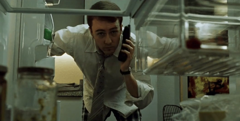
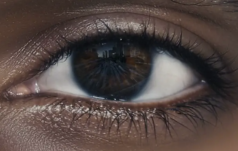
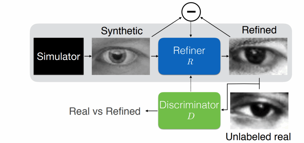
- gaze estimation means tracking where exactly you are looking at on the screen; right now gaze estimation is important for focus group studies intended to design better interfaces and more efficient advertising, but I expect that in the near future it will be a key technology for a wide range of user-facing AR/VR applications;
- emotion recognition has obvious applications in finding out user reactions to interactions with automated systems and less obvious but perhaps even more important applications such as recognizing whether a car driver is about to fall asleep behind the wheel;
- all of these problems may include and rely upon facial keypoint recognition, that is, finding specific points of interest on a human face, and so on, and so forth.
Synthetic models and images of people (both faces and full bodies) are an especially interesting subject for synthetic data. On the one hand, while large-scale real datasets of photographs of humans definitely exist they are even harder to collect. First, there are privacy issues involved in the collection of real human faces; I will postpone this discussion until a separate post on synthetic faces, so let me just link to a recent study by Raji and Fried (2021) who point out a lot of problems in this regard within existing large-scale datasets.
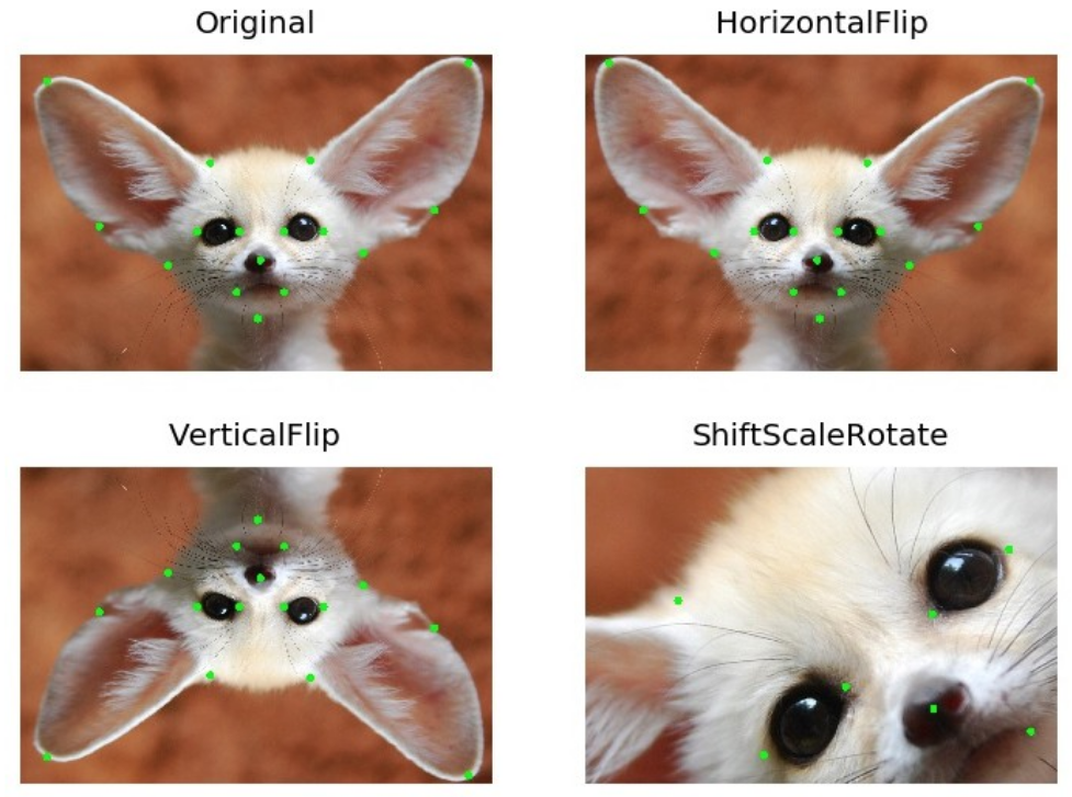
Second, the labeling for some basic computer vision problems is especially complex: while pose estimation is doable, facial keypoint detection (a key element for facial recognition and image manipulation for faces) may require to specify several dozen landmarks on a human face, which becomes very hard for human labeling.
Third, even if a large dataset is available, it often contains biases in its composition of genders, races, or other parameters of human subjects, sometimes famously so; again, for now let me just link to a paper by Kortylewski et al. (2017) that we will discuss in detail in a later post.
These are the primary advantages of using synthetic datasets for human faces (beyond the usual reasons such as limitless perfectly labeled data). On the other hand, there are complications as well, chief of them being that synthetic 3D models of people and especially synthetic faces are much harder to create than models of basic objects, especially if sufficient fidelity is required. This creates a tension between the quality of available synthetic faces and improvements in face recognition and other related tasks that they can provide.
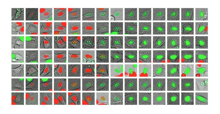
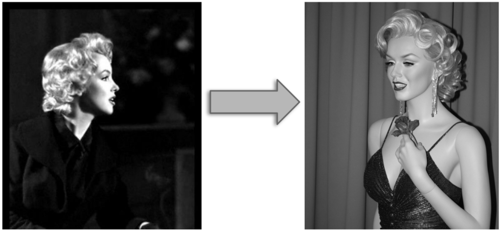
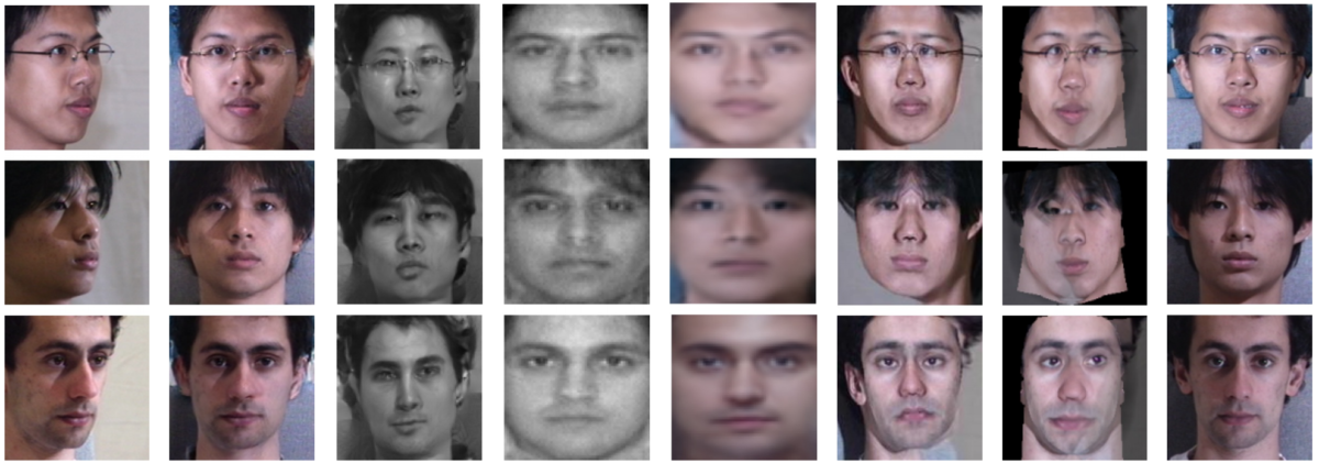
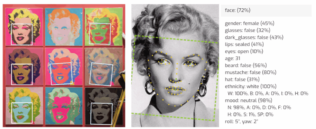
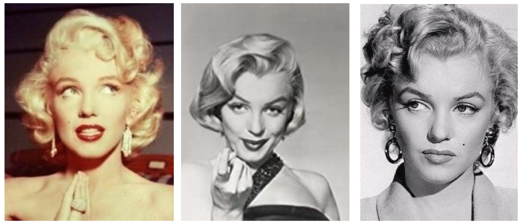
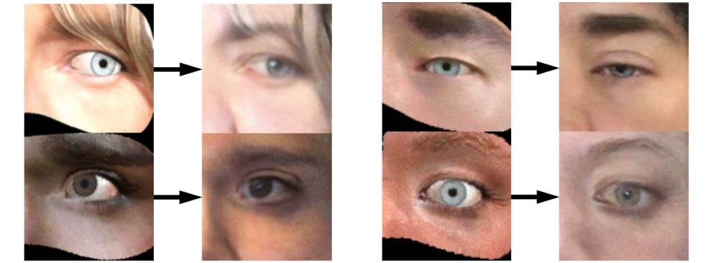
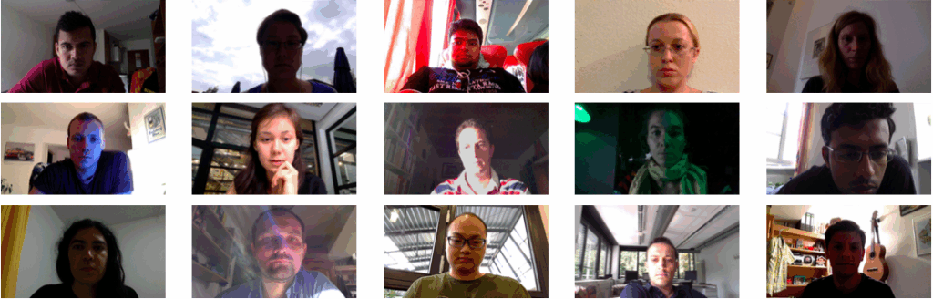
Here at Synthesis AI, we have already developed a system for producing large-scale synthetic datasets of human faces, including very detailed labeling of facial landmarks, possible occlusions such as glasses or medical masks, varying lighting conditions, and much more. Again, we will talk about this in much more detail later, so for now let me show a few examples of what our APIs are capable of and go on to the next application.
Indoor Environments
Human faces seldom require simulation environments because most applications, including all listed above, deal with static pictures and will not benefit much from a video. But in our next set of examples, it is often crucial to have an interactive environment. Static images will hardly be sufficient to train, e.g., an autonomous vehicle such as a self-driving car or a drone, or an industrial robot. Learning to control a vehicle or robot often requires reinforcement learning, where an agent has to learn from interacting with the environment, and real world experiments are usually entirely impractical for training. Fortunately, this is another field where synthetic data shines: once one has a fully developed 3D environment that can produce datasets for computer vision or other sensory readings, it is only one more step to begin active interaction or at least movement within this environment.
We begin with indoor navigation, an important field where synthetic datasets are required. The main problems here are, as usual for such environments, SLAM (simultaneous localization and mapping, i.e., understanding where the agent is located inside the environment) and navigation. Potential applications here lie in the field of home robotics, industrial robots, and embodied AI, but for our purposes you can simply think of a robotic vacuum cleaner that has to navigate your house based on sensor readings. There exist large-scale efforts to create real annotated datasets of indoor scenes (Chang et al., 2017; Song et al., 2015; Xia et al., 2018), but synthetic data has always been extremely important.
Historically, the main synthetic dataset for indoor navigation was SUNCG4 presented by Song et al. (2017).
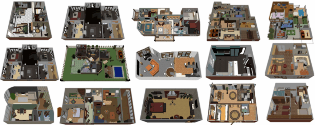
It contained over 45,000 different scenes (floors of private houses) with manually created realistic room layouts, 3D models of the furniture, realistic textures, and so on. All scenes were semantically annotated at the object level, and the dataset provides synthetic depth maps and volumetric ground truth data for the scenes. The original paper presented state of the art results in semantic scene completion, but, naturally, SUNCG has been used for many different tasks related to depth estimation, indoor navigation, SLAM, and others; see Qi et al. (2017), Abbasi et al. (2018), and Chen et al. (2019), to name just a few. It often served as the basis for scene understanding competitions, e.g., the 2019 SUMO workshop at CVPR 2019 on 360° Indoor Scene Understanding and Modeling.
Why the past tense, though? Interestingly, even indoor datasets without any humans in them can be murky in terms of legality. Right now, the SUNCG paper website is up but the dataset website is down and SUNCG itself is unavailable due to a legal controversy over the data: the Planner5D company claims that Facebook used their software and data to produce SUNCG and made it publicly available without consent from Planner5D; see more details here.
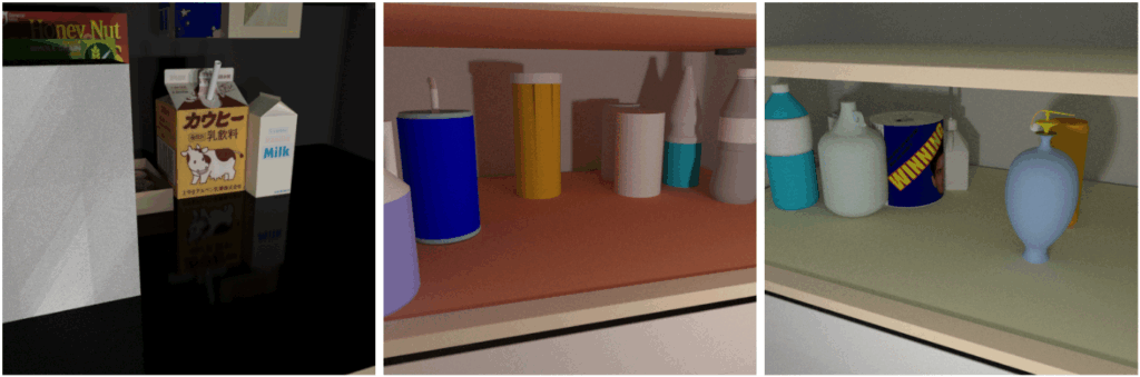
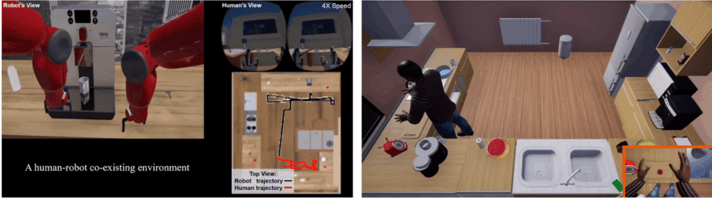
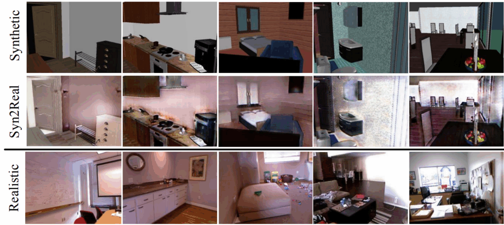
In any case, by now we have larger and more detailed synthetic indoor environments. A detailed survey will have to wait for a separate post, but I want to highlight the AI Habitat released by the very same Facebook; see also the paper by Savva, Kadian et al. (2019). It is a simulated environment explicitly intended to trained embodied AI agents, and it includes a high-performance full 3D simulator with high-fidelity images. AI Habitat environments might look something like this:
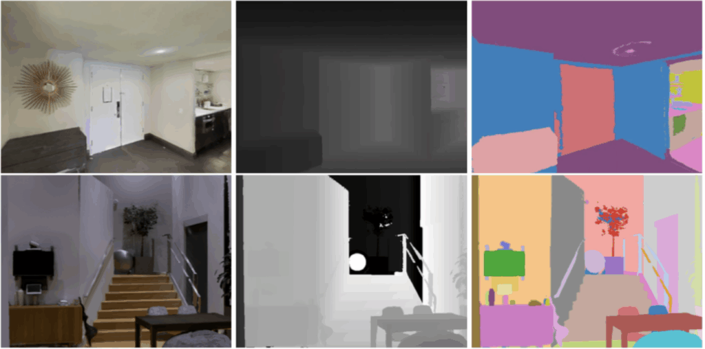
Simulated environments of this kind can be used to train home robots, security cameras, and AI assistants, develop AR/VR applications, and much more. It is an exciting field where Synthesis AI is also making advances to.
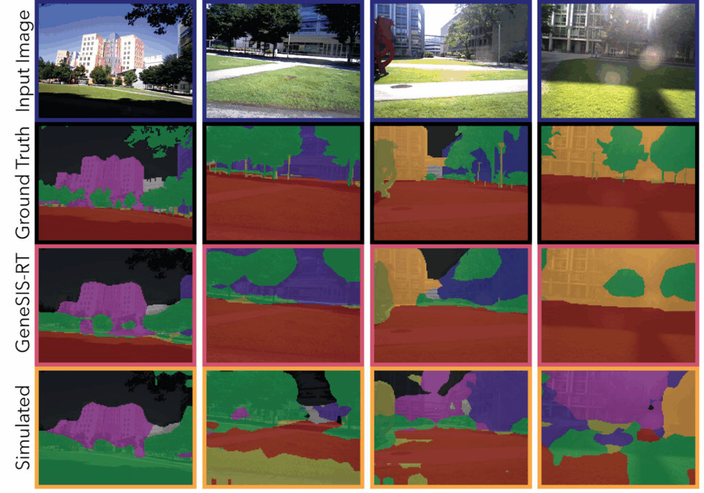
Outdoor Environments
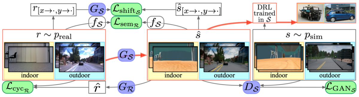
Now we come to one of the most important and historically best developed directions of applications for synthetic data: outdoor simulated environments intended to improve the motion of autonomous robots. Possible applications include SLAM, motion planning, and motion for control for self-driving cars (urban navigation), unmanned aerial vehicles, and much more (Fossen et al., 2017; Milz et al., 2018; Paden et al., 2016); see also general surveys of computer vision for mobile robot navigation (Bonin-Font et al., 2008; Desouza, Kak, 2002) and perception and control for autonomous driving (Pendleton et al., 2017).
There are two main directions here:
- training vision systems for segmentation, SLAM, and other similar problems; in this case, synthetic data can be represented by a dataset of static images;
- fully training autonomous driving agents, usually with reinforcement learning, in a virtual environment; in this case, you have to be able to render the environment in real time (preferably much faster since reinforcement learning usually needs millions of episodes), and the system also has to include a realistic simulation of the controls for the agent.
I cannot hope to give this topic justice in a single section, so there will definitely be separate posts on this, and for now let me just scatter a few examples of modern synthetic datasets for autonomous driving.
First, let me remind you that one of the very first applications of synthetic data to training neural networks, the ALVINN network that we already discussed on this blog, was actually an autonomous driving system. Trained on synthetic 30×32 videos supplemented with 8×32 range finder data, ALVINN was one of the first successful applications of neural networks in autonomous driving.
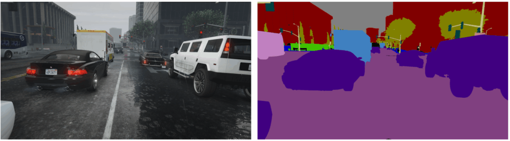
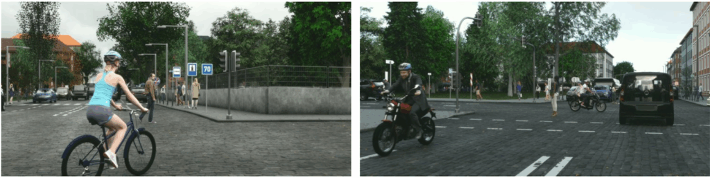
By now, resolutions have grown. Around 2015-2016, researchers realized that modern interactive 3D projects (that is, games) had progressed so much that one can use their results as high-fidelity synthetic data. Therefore, several important autonomous driving datasets produced at that time used modern 3D engines such as Unreal Engine or even specific game engines such as Grand Theft Auto V to generate their data. Here is a sample from the GTAV dataset by Richter et al. (2016):
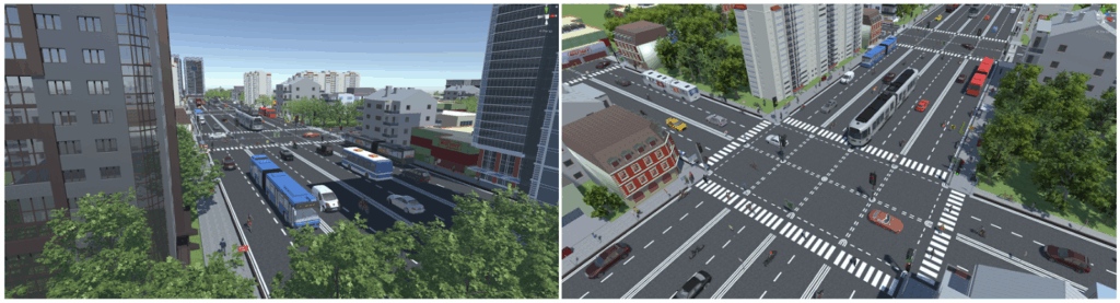
And here is a sample from the VEIS dataset by Saleh et al. (2018) who used Unity 3D:
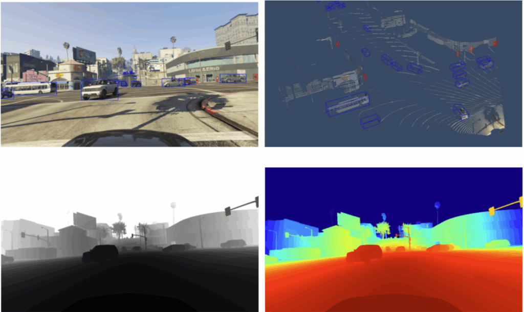
For the purposes of synthetic data, researchers often had to modify CGI and graphics engines to suit machine learning requirements, especially to implement various kinds of labeling. For example, the work based on Grand Theft Auto V was recently continued by Hurl et al. (2019) who developed a precise LIDAR simulator within the GTA V engine and published the PreSIL (Precise Synthetic Image and LIDAR) dataset with over 50000 frames with depth information, point clouds, semantic segmentation, and detailed annotations. Here is a sample of just a few of its modalities:
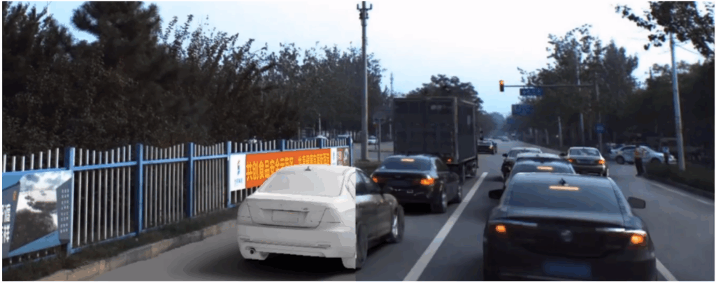
Another interesting direction was pursued by Li et al. (2019) who developed the Augmented Autonomous Driving Simulation (AADS) environment. This synthetic data generator is able to insert synthetic traffic on real-life RGB images in a realistic way. With this approach, a single real image can be reused many times in different synthetic traffic situations. Here is a sample frame from the AADS introductory video that emphasizes that the cars are synthetic — otherwise you might well miss it!
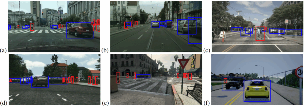
Fully synthetic datasets are also rapidly approaching photorealism. In particular, the Synscapes dataset by Wrenninge and Unger (2018) is quite easy to take for real at first glance; it simulates motion blur and many other properties of real photographs:
Naturally, such photorealistic datasets cannot be rendered in full real time yet, so they usually represent collections of static images. Let us hope that cryptocurrency mining will leave at least a few modern GPUs to advance this research, and let us proceed to our next item.
Industrial Simulated Environments
Imagine a robotic arm manipulating items on an assembly line. Controlling this arm certainly looks like a machine learning problem… but where will the dataset come from? There is no way to label millions of training data instances, especially once you realize that the function that we are actually learning is mapping activations of the robot’s drives and controls into reactions of the environment.
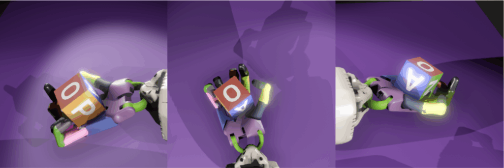
Consider, for instance, the Dactyl robot that OpenAI researchers recently taught to solve a Rubik’s cube in real life (OpenAI, 2018). It was trained by reinforcement learning, which means that the hand had to make millions, if not billions, of attempts at interacting with the environment. Naturally, this could be made possible only by a synthetic simulation environment, in this case ORRB (OpenAI Remote Rendering Backend) also developed by OpenAI (Chociej et al., 2019). For a robotic hand like Dactyl, ORRB can very efficiently render views of randomized environments that look something like this:
And that’s not all: to be able to provide interactions that can serve as fodder for reinforcement learning, the environment also has to implement a reasonably realistic physics simulator. Robotic simulators are a venerable and well-established field; the two most famous and most popular engines are Gazebo, originally presented by Koenig and Howard (2004) and currently being developed by Open Source Robotics Foundation (OSRF), and MuJoCo (Multi-Joint Dynamics with Contact) developed by Todorov et al. (2012); for example, ORRB mentioned above can interface with MuJoCo to provide an all-around simulation.
This does not mean that new engines cannot arise for robotics. For example, Xie et al. (2019) presented VRGym, a virtual reality testbed for physical and interactive AI agents. Their main difference from previous work is the support of human input via VR hardware integration. The rendering and physics engine are based on Unreal Engine 4, and additional multi-sensor hardware is capable of full body sensing and integration of human subjects to virtual environments. Moreover, a special bridge allows to easily communicate with robotic hardware, providing support for ROS (Robot Operating System), a standard set of libraries for robotic control. Visually it looks something like this:
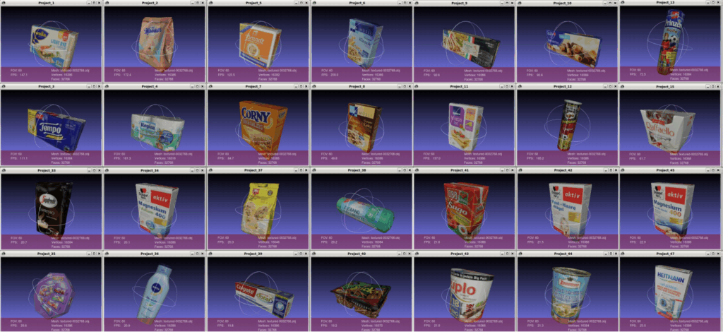
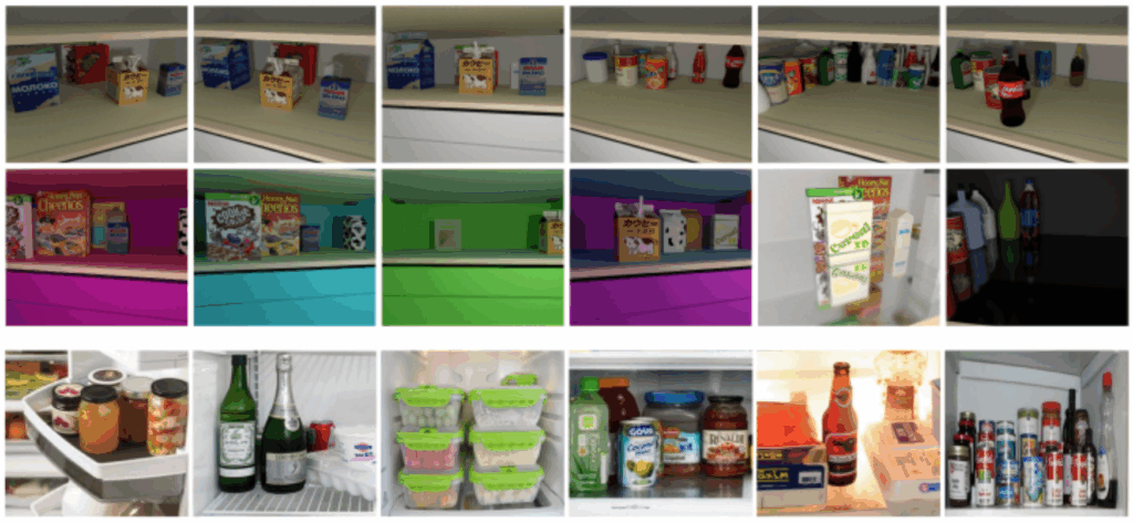
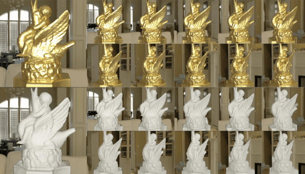
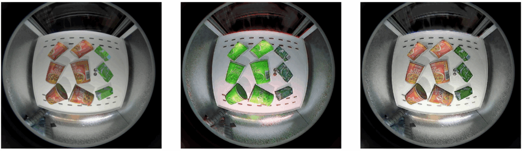
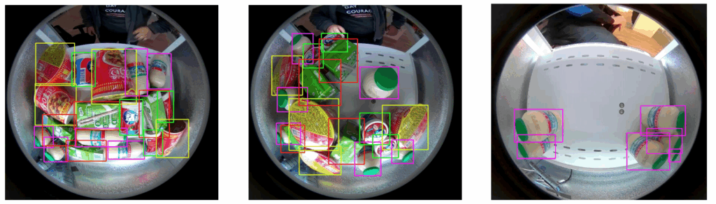
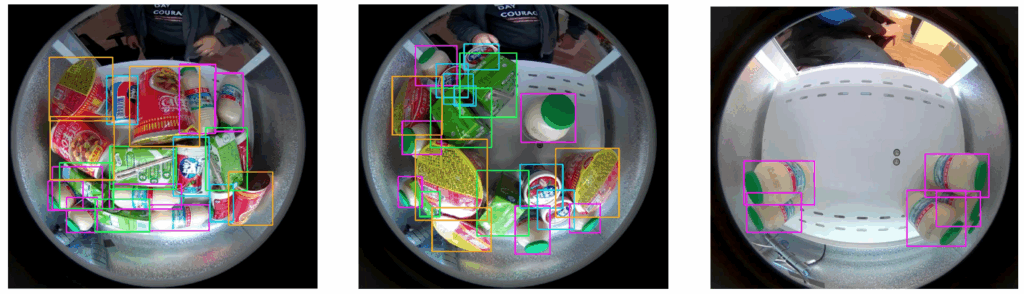
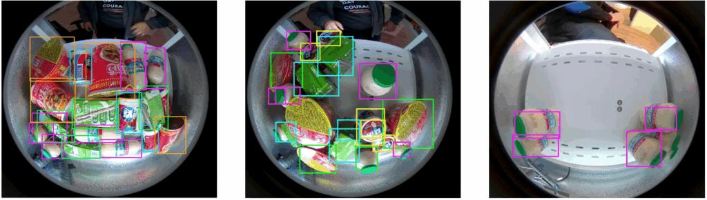
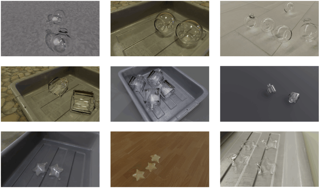
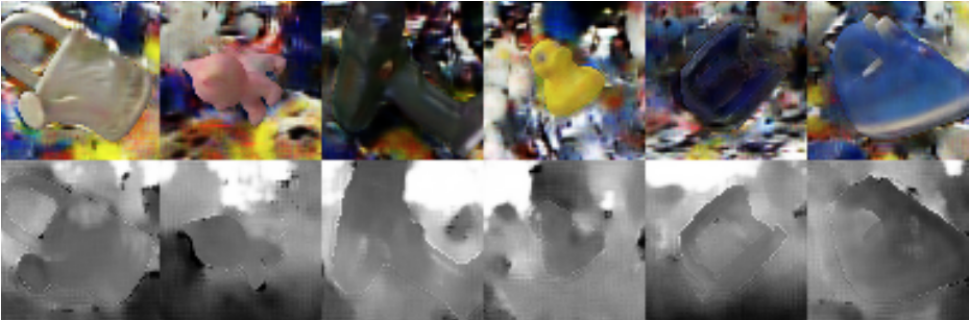
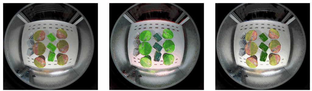
Here at Synthesis AI, we are already working in this direction. In a recent collaboration with Google Robotics called ClearGrasp (we covered it on the blog a year ago), we developed a large-scale dataset of transparent objects that present special challenges for computer vision: transparent objects are notoriously hard for object detection, depth estimation, and basically any computer vision task you can think of. With the help of this dataset, in the ClearGrasp project we developed machine learning models capable of estimating accurate 3D data of transparent objects from RGB-D images. The dataset looks something like this, and for more details I refer to our earlier post and to Google’s web page on the ClearGrasp project:
There is already no doubt that end-to-end training of industrial robots is virtually impossible without synthetic environments. Still, I believe there is a lot to be done here, both specifically for robotics and generally for the best adaptation and usage of synthetic environments.
Synthetic Documents and Media
Finally, we come to the last item in the post: synthetic documents and media. Let us begin with optical character recognition (OCR), which mostly means reading the text written on a photo, although there are several different tasks related to text recognition: OCR itself, text detection, layout analysis and text line segmentation for document digitization, and others.
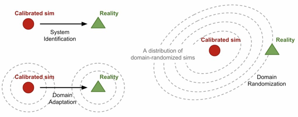
The basic idea for synthetic data in OCR is simple: it is very easy to produce synthetic text, so why don’t we superimpose synthetic text on real images, or simply on varied randomized backgrounds (recall our discussion of domain randomization), and train on that? Virtually all modern OCR systems have been trained on data produced by some variation of this idea.
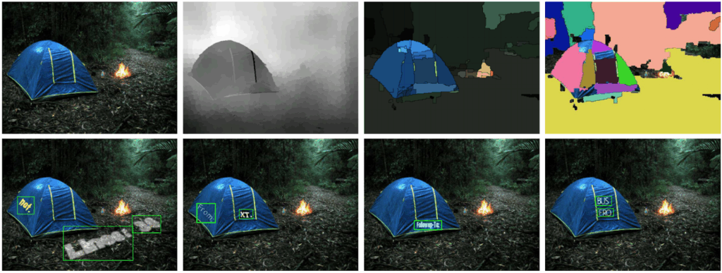
I will highlight the works where text is being superimposed in a “smarter”, more realistic way. For instance, Gupta et al. (2016) in their SynthText in the Wild dataset use depth estimation and segmentation models to find regions (planes) of a natural image suitable for placing synthetic text, and even find the correct rotation of text for a given plane. This process is illustrated in the top row of the sample image, and the bottom row shows sample text inserted onto suitable regions:
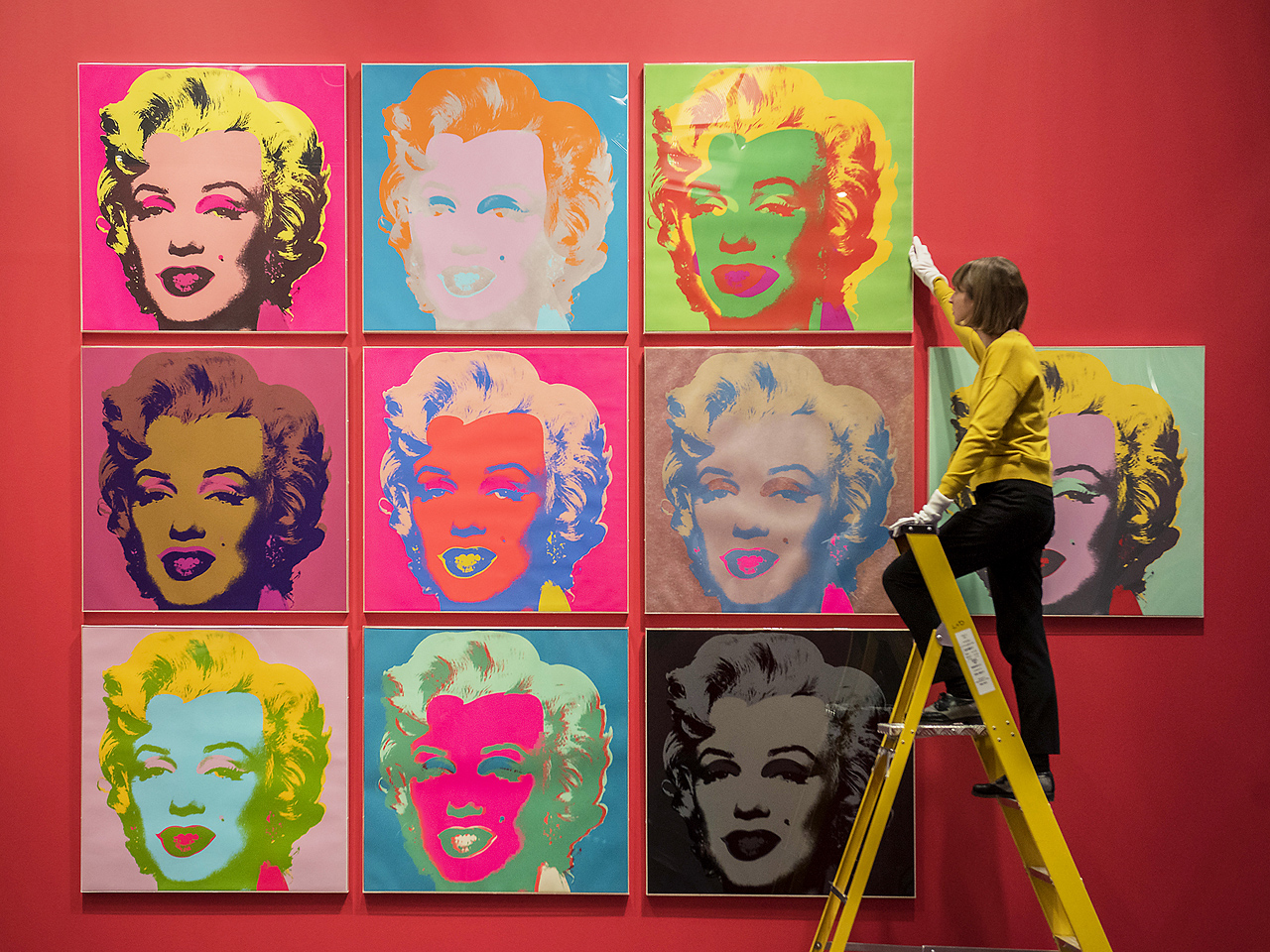
Another interesting direction where such systems might go (but have not gone yet) is the generation of synthetic media that includes text but is not limited to it. Currently, advertising and rich media in general are at the frontier of multimodal approaches that blend together computer vision and natural language processing. Think about the rich symbolism that we see in many modern advertisements; sometimes understanding an ad borders on a lateral thinking puzzle. For instance, what does this image advertise?
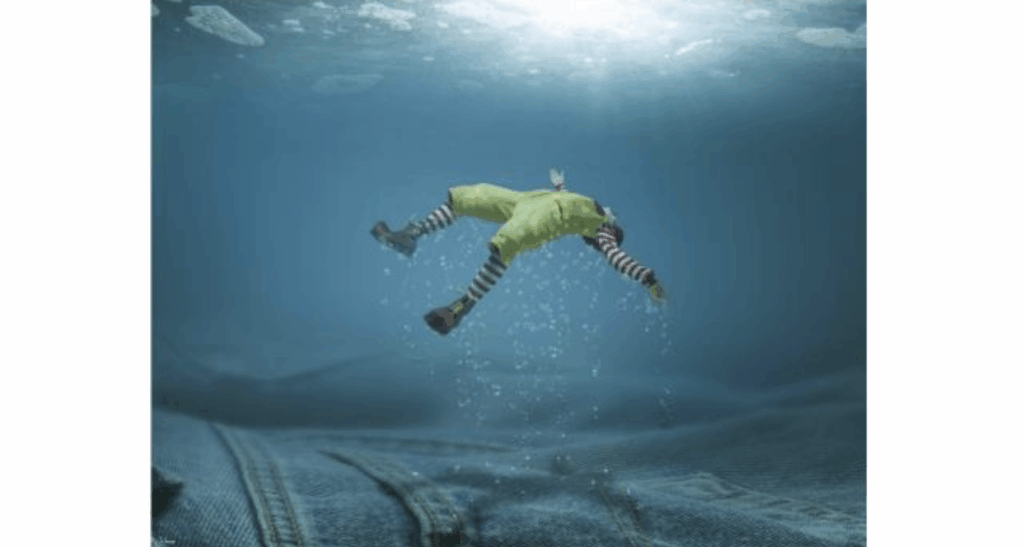
The answer is explicitly stated in the slogan that I’ve cut off: “Removes fast food stains fast”. You might have got it instantaneously, or you might have had to think for a little bit, but how well do you think automated computer vision models can pick up on this? This is a sample image from the dataset collected by researchers from the University of Pittsburgh. Understanding this kind of symbolism is very hard, and I can’t imagine generating synthetic data for this problem at this point.
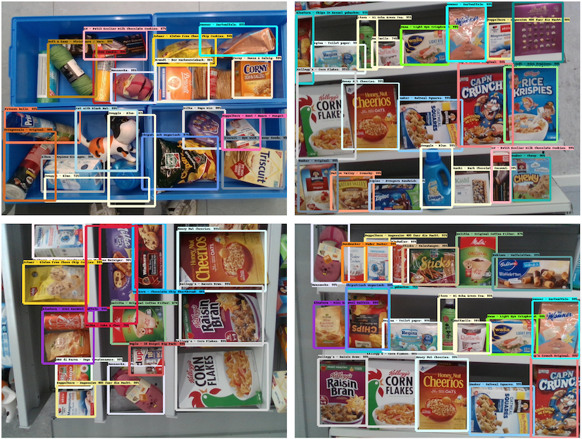
But perhaps easier questions would include at least detecting advertisements in our surroundings, detecting logos and brand names in the advertising, reading the slogans, and so on. Here, a synthetic dataset is not hard to imagine; at the very least, we could cut off ads from real photos and paste other ads in their place. But even solving this restricted problem would be a huge step forward for AR systems! If you are an advertiser, imagine that you can insert ads in augmented reality on the fly; and if you are just a regular human being imagine that you can block off real life ads or replace them with pleasing landscape photos as you go down the street. This kind of future might be just around the corner, and it might be helped immensely by synthetic data generation.
Conclusion
In this (rather long) post, I’ve tried to give a brief overview of the main directions where we envision the present and future of synthetic data for machine learning. Here at Synthesis AI, we are working to bring this vision of the future to reality. In the next post of this series, we will go into more detail about one of these use cases and showcase some of our work.
Sergey Nikolenko
Head of AI, Synthesis AI

![\[\min_{\theta_G,\theta_T}\;\max_{\phi}\;\lambda_{1}\,\mathcal{L}_{\text{dom}}^{\text{PIX}}(D^{\text{PIX}},G^{\text{PIX}})+\lambda_{2}\,\mathcal{L}_{\text{task}}^{\text{PIX}}(G^{\text{PIX}},T^{\text{PIX}})+\lambda_{3}\,\mathcal{L}_{\text{cont}}^{\text{PIX}}(G^{\text{PIX}}),\]](https://blog.sergeynikolenko.ru/wp-content/ql-cache/quicklatex.com-957dcb2f206295ade0efd10261988ed3_l3.svg "Rendered by QuickLaTeX.com")
![\begin{align*}\mathcal{L}_{\text{dom}}^{\text{PIX}}(D^{\text{PIX}},G^{\text{PIX}}) =&\mathbb{E}_{\mathbf{x}_{S}\sim p_{\text{syn}}}\!\bigl[\log\!\bigl(1-D^{\text{PIX}}\!\bigl(G^{\text{PIX}}(\mathbf{x}_{S};\theta_{G});\phi\bigr)\bigr)\bigr]\\ +&\mathbb{E}_{\mathbf{x}_{T}\sim p_{\text{real}}}\!\bigl[\log D^{\text{PIX}}(\mathbf{x}_{T};\phi)\bigr];\end{align*}](https://blog.sergeynikolenko.ru/wp-content/ql-cache/quicklatex.com-efef45d7c7e94718bc3c779ccbd18aa7_l3.svg "Rendered by QuickLaTeX.com")
![\begin{align*}\mathcal{L}_{\text{task}}^{\text{PIX}}&(G^{\text{PIX}},T^{\text{PIX}}) = \\ &\mathbb{E}_{\mathbf{x}_{S},\mathbf{y}_{S}\sim p_{\text{syn}}} \!\bigl[-\mathbf{y}_{S}^{\top}\!\log T^{\text{PIX}}\!\bigl(G^{\text{PIX}}(\mathbf{x}_{S};\theta_{G});\theta_{T}\bigr) -\mathbf{y}_{S}^{\top}\!\log T^{\text{PIX}}(\mathbf{x}_{S};\theta_{T})\bigr],\end{align*}](https://blog.sergeynikolenko.ru/wp-content/ql-cache/quicklatex.com-b6a76786421e6e623da00bc4631f9bda_l3.svg "Rendered by QuickLaTeX.com")
![\begin{align*}\mathcal{L}_{\text{cont}}^{\text{PIX}}(G^{\text{PIX}}) =\mathbb{E}_{\mathbf{x}_{S}\sim p_{\text{syn}}}\!\Bigl[& \frac{1}{k}\,\lVert(\mathbf{x}_{S}-G^{\text{PIX}}(\mathbf{x}_{S};\theta_{G}))\odot m(\mathbf{x})\rVert_{2}^{2}\\ &-\frac{1}{k^{2}}\bigl((\mathbf{x}_{S}-G^{\text{PIX}}(\mathbf{x}_{S};\theta_{G}))^{\top}m(\mathbf{x})\bigr)^{2} \Bigr],\end{align*}](https://blog.sergeynikolenko.ru/wp-content/ql-cache/quicklatex.com-9b49079973db116b7c3f74dc0090161b_l3.svg "Rendered by QuickLaTeX.com")
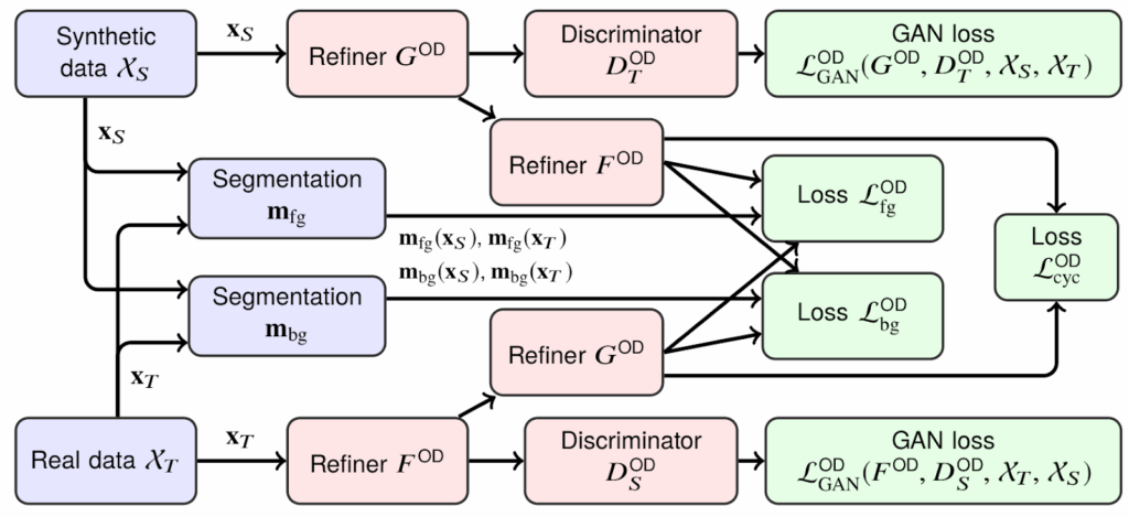
 is a segmentation mask for the foreground object extracted from the synthetic data renderer; note that this loss does not “insist” on preserving pixel values in the object but rather encourages the model to change object pixels in a consistent way, preserving their pairwise differences.
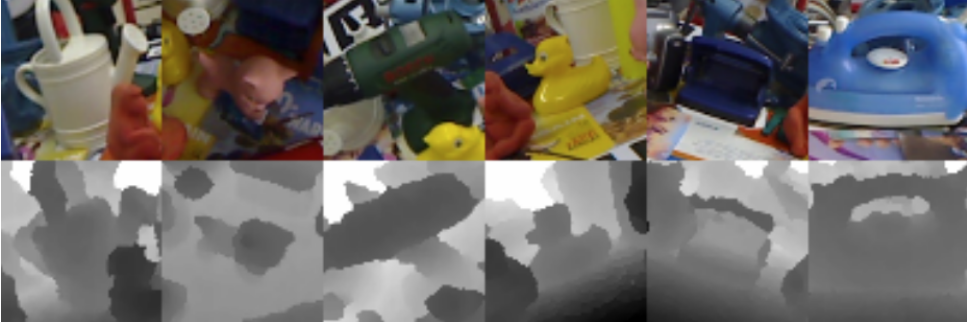

![\[\mathcal{L}^{T2}=\mathcal{L}_{\text{GAN}}^{T2}(G_{S}^{T2},D_{T}^{T2})+\lambda_{1}\mathcal{L}_{\text{GAN}_f}^{T2}(f_{\text{task}}^{T2},D_{f}^{T2})+\lambda_{2}\mathcal{L}_{r}^{T2}(G_{S}^{T2})+\lambda_{3}\mathcal{L}_{t}^{T2}(f_{\text{task}}^{T2})+\lambda_{4}\mathcal{L}_{s}^{T2}(f_{\text{task}}^{T2}),\]](https://blog.sergeynikolenko.ru/wp-content/ql-cache/quicklatex.com-0993df42fb2d0258cab8f36cab798906_l3.svg "Rendered by QuickLaTeX.com")
![\begin{align*}\mathcal{L}_{\text{GAN}}^{T2}(G_{S}^{T2},D_{T}^{T2}) =&\mathbb{E}_{\mathbf{x}_{S}\sim p_{\text{syn}}} \bigl[\log(1-D_{T}^{T2}(G_{S}^{T2}(\mathbf{x}_{S})))\bigr]\\ +&\mathbb{E}_{\mathbf{x}_{T}\sim p_{\text{real}}} \bigl[\log D_{T}^{T2}(\mathbf{x}_{T})\bigr];\end{align*}](https://blog.sergeynikolenko.ru/wp-content/ql-cache/quicklatex.com-1633b4a1cb54b96701fbe567dda9832b_l3.svg "Rendered by QuickLaTeX.com")
![\begin{align*}\mathcal{L}_{\text{GAN}_f}^{T2}(f_{\text{task}}^{T2},D_{f}^{T2}) &=\mathbb{E}_{\mathbf{x}_{S}\sim p_{\text{syn}}} \bigl[\log D_{f}^{T2}(f_{\text{task}}^{T2}(G_{S}^{T2}(\mathbf{x}_{S})))\bigr]\\ &+\mathbb{E}_{\mathbf{x}_{T}\sim p_{\text{real}}} \bigl[\log(1-D_{f}^{T2}(f_{\text{task}}^{T2}(\mathbf{x}_{T})))\bigr]; \end{align*}](https://blog.sergeynikolenko.ru/wp-content/ql-cache/quicklatex.com-3df7b15dd51e4530b11b26b512dcab70_l3.svg "Rendered by QuickLaTeX.com")
 is the reconstruction loss for real images, simply an
  norm that says that T2Net is not supposed to change real images at all;
 is the task loss for depth estimation on synthetic images, namely the
  is the task loss for depth estimation on real images:
![\[\mathcal{L}_{s}^{T2}(f_{\text{task}}^{T2}) = |\partial_{x} f_{\text{task}}^{T2}(\mathbf{x}_{T})|^{-|\partial_{x}\mathbf{x}_{T}|} + |\partial_{y} f_{\text{task}}^{T2}(\mathbf{x}_{T})|^{-|\partial_{y}\mathbf{x}_{T}|},\]](https://blog.sergeynikolenko.ru/wp-content/ql-cache/quicklatex.com-6beff73b968312ed5f48a71d5509cc02_l3.svg "Rendered by QuickLaTeX.com")


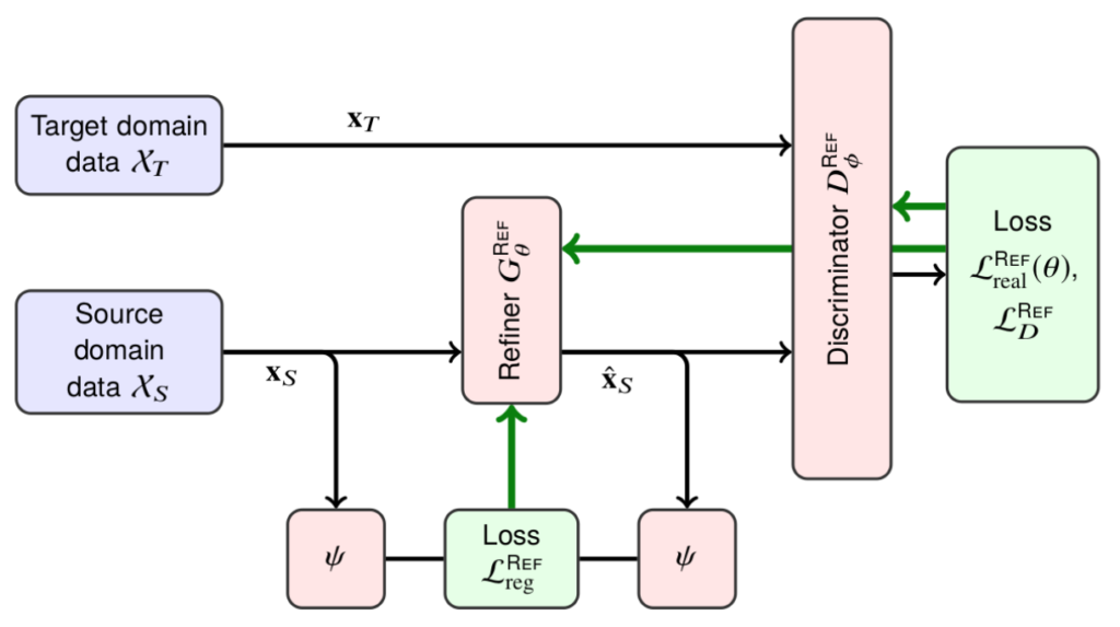
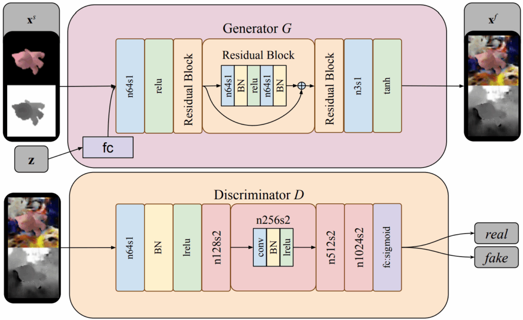
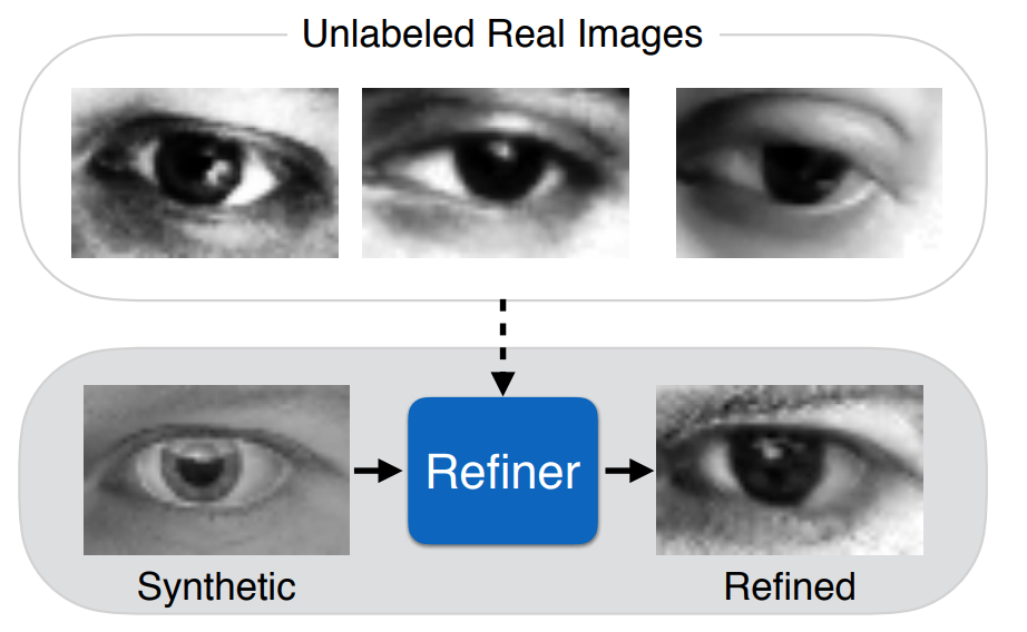
![\begin{align*}\mathcal{L}^{\text{REF}}_{G}(\theta) &= \mathbb{E}_{S}\Bigl[ \mathcal{L}^{\text{REF}}_{\text{real}}\!\bigl(\theta;\mathbf{x}_{S}\bigr) + \lambda\, \mathcal{L}^{\text{REF}}_{\text{reg}}\!\bigl(\theta;\mathbf{x}_{S}\bigr) \Bigr], \quad\text{where} \\[6pt]\mathcal{L}^{\text{REF}}_{\text{real}}\!\bigl(\theta;\mathbf{x}_{S}\bigr) &= -\,\log\!\Bigl(1 - D^{\text{REF}}_{\phi}\bigl(G^{\text{REF}}_{\theta}(\mathbf{x}_{S})\bigr)\Bigr), \\[6pt]\mathcal{L}^{\text{REF}}_{\text{reg}}\!\bigl(\theta;\mathbf{x}_{S}\bigr) &= \bigl\lVert \psi\!\bigl(G^{\text{REF}}_{\theta}(\mathbf{x}_{S})\bigr) - \psi(\mathbf{x}_{S}) \bigr\rVert_{1}\;.\end{align*}](https://blog.sergeynikolenko.ru/wp-content/ql-cache/quicklatex.com-5377b2ebb38f4ac4573f3e99f49cf12b_l3.svg "Rendered by QuickLaTeX.com")
 is a mapping into some kind of feature space. The feature space can contain the image itself, image derivatives, statistics of color channels, or features produced by a fixed extractor such as a pretrained CNN. But in case of SimGAN it was… in most cases, just an identity map. That is, the regularization loss simply told the generator to change as little as possible while still making the image realistic.
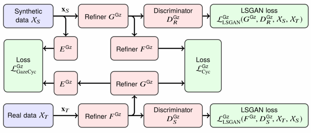
 and
and  , and two discriminators, one for the source domain and one for the target domain. What’s going on here?
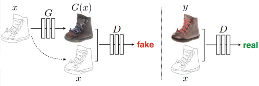

 can be a simple
  or
or 
![\begin{align*}\mathcal{L}_{\text{Cyc}}^{Gz}\!\bigl(G^{Gz},F^{Gz}\bigr) =& \mathbb{E}_{\mathbf{x}_{S}\sim p_{\text{syn}}} \!\Bigl[\bigl\|F^{Gz}\!\bigl(G^{Gz}(\mathbf{x}_{S})\bigr)-\mathbf{x}_{S}\bigr\|_{1}\Bigr]\\ +&\mathbb{E}_{\mathbf{x}_{T}\sim p_{\text{real}}} \!\Bigl[\bigl\|G^{Gz}\!\bigl(F^{Gz}(\mathbf{x}_{T})\bigr)-\mathbf{x}_{T}\bigr\|_{1}\Bigr];\end{align*}](https://blog.sergeynikolenko.ru/wp-content/ql-cache/quicklatex.com-a6479de0e633a11dae48f110a0f75e2b_l3.svg "Rendered by QuickLaTeX.com")
![\[\mathcal{L}_{\text{GazeCyc}}^{Gz}\bigl(G^{Gz},F^{Gz}\bigr) = \mathbb{E}_{\mathbf{x}_S\sim p_{\text{syn}}}\left[\left\| E^{Gz}\left(F^{Gz}(G^{Gz}(\mathbf{x}_S))\right) - E^{Gz}(\mathbf{x}_S)\right\|_2^2\right].\]](https://blog.sergeynikolenko.ru/wp-content/ql-cache/quicklatex.com-7ec6f9195cd5251a6e1ddcd68cabef95_l3.svg "Rendered by QuickLaTeX.com")
![\begin{align*}\min_{D}\; V_{\text{LSGAN}}(D)&= \tfrac12\,\mathbb{E}_{\mathbf{x}\sim p{\text{data}}}\bigl[(D(\mathbf{x}) - b)^{2}\bigr]+ \tfrac12\,\mathbb{E}_{\mathbf{z}\sim p{z}}\bigl[(D(G(\mathbf{z})) - a)^{2}\bigr], \\\min_{G}\; V_{\text{LSGAN}}(G)&= \tfrac12\,\mathbb{E}_{\mathbf{z}\sim p{z}}\bigl[(D(G(\mathbf{z})) - c)^{2}\bigr],\end{align*}](https://blog.sergeynikolenko.ru/wp-content/ql-cache/quicklatex.com-17085664f89788591d5bd50a9582c94f_l3.svg "Rendered by QuickLaTeX.com")
 on real images and some other constant
  on fake images, while the generator is trying to convince the discriminator to output c on fake images (it has no control over the real ones). Naturally, usually one takes
  and
and  , although there is an interesting theoretical result about the case when
  and
and  , that is, when the generator is trying to make the discriminator maximally unsure about the fake images.
![\[\mathcal{L}_{\text{LSGAN}}^{Gz}(G, D, S, R) = \mathbb{E}_{\mathbf{x}_S \sim p{_\text{syn}}}\Bigl[\,\bigl(D\bigl(G(\mathbf{x}_S)\bigr) - 0.9\bigr)^{2}\Bigr] + \mathbb{E}_{\mathbf{x}_T \sim p_{\text{real}}}\Bigl[\,D(\mathbf{x}_T)^{2}\Bigr];\]](https://blog.sergeynikolenko.ru/wp-content/ql-cache/quicklatex.com-2c73a446a0e5b4c80b7031df6b98840f_l3.svg "Rendered by QuickLaTeX.com")


![\begin{align*}\tilde{x} &= \lambda x_i + (1 - \lambda) x_j,&\text{where } x_i, x_j \text{ are raw input vectors,} \\[4pt]\tilde{y} &= \lambda y_i + (1 - \lambda) y_j,&\text{where } y_i, y_j \text{ are one-hot label encodings.}\end{align*}](https://blog.sergeynikolenko.ru/wp-content/ql-cache/quicklatex.com-dc7c242c1407bae338fe0bb1b9014ef1_l3.svg "Rendered by QuickLaTeX.com")