Convolutional Networks

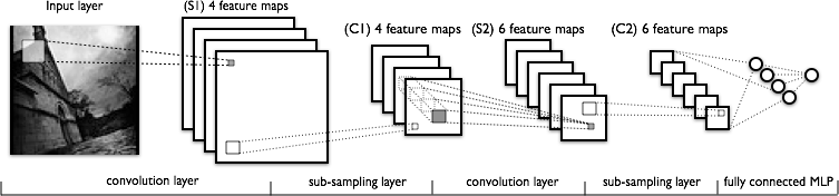
And now let us turn to convolutional networks. In 1998, the French computer scientist Yann LeCun presented the architecture of a convolutional neural network (CNN).

The network is named after the mathematical operation of convolution, which is often used for image processing and can be expressed by the following formula:

   

where  is the original matrix of the image, and  is the convolution kernel (convolution matrix).

The basic assumption is that the input is not a discrete set of independent dimensions but rather an actual image where the relative placement of the pixels is crucial,. Certain pixels are positioned close to one another, while others are far away. In a convolutional neural network one second-layer neuron is linked to some of the first-layer neurons that are located close together, not all of them. Then these neurons will gradually learn to recognize local features. Second-layer neurons designed in the same way will respond to local combinations of local first-layer features and so on. A convolutional network almost always consists of multiple layers, up to about a dozen in early CNNs and up to hundreds and even thousands now.

Each layer of a convolutional network consists of three operations:

• the convolution, which we have just described above,
• non-linearity such as a sigmoid function or a hyperbolic tangent,
• and pooling (subsampling).

Pooling, also known as subsampling, applies a simple mathematical function (mean, max, min…) to a local group of neurons. In most cases, it’s considered more important for higher-layer neurons to check whether or not a certain feature is in an area than to remember its precise coordinates. The most popular form of pooling is max-pooling: the higher level neuron activates if at least one neuron it its corresponding window activated. Among other things, this approach enables you to make the convolutional network resistant to small changes.

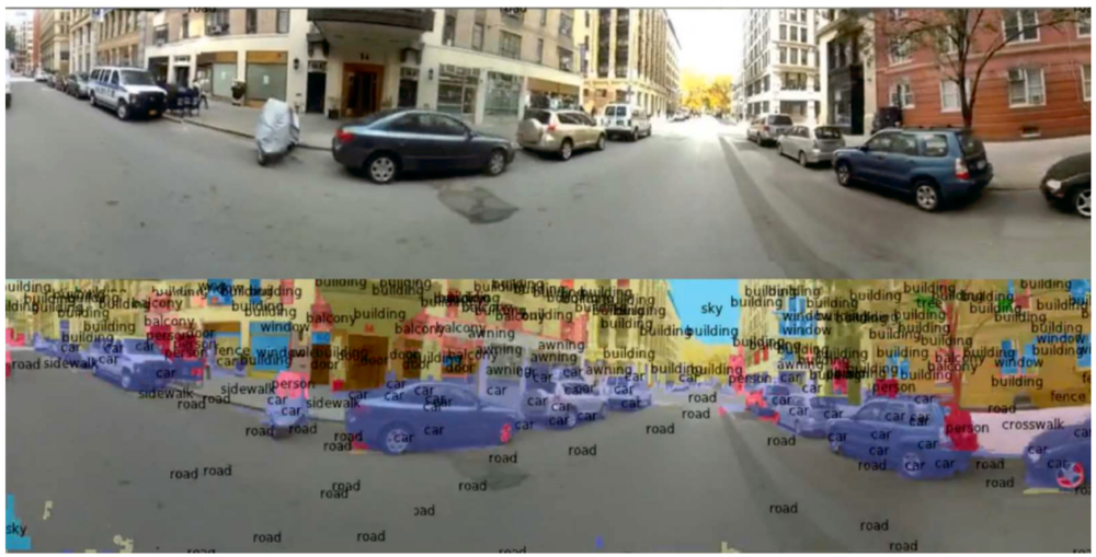
Numerous modern computer vision applications run on convolutional networks. For instance, Prisma, the app you’ve probably heard about runs on convolutional neural networks. Practically all modern computer visual apps use convolutional networks for recognizing objects on images. For instance, CNN-based scene labeling solutions, where an image from a camera is automatically divided into different zones classified as known objects like “pavement”, “car”, or “tree”, underlie driver assistance systems. Actually, the drivers aren’t always necessary: the same kind of networks are now used for creating self-driving cars.

Reinforcement Learning

Generally, machine learning tasks are divided into two types — supervised learning, when the correct answers are already given and the machine learns based on them, and unsupervised learning, when the questions are given but the answers aren’t. Things look different in real life. How does a child learn? When she walks into a table and hits her head, a signal saying, “Table means pain,” goes to her brain. The child won’t smack her head on the table the next time (well, maybe two times later). In other words, the child actively explores her environment without having received any correct answers. The brain doesn’t have any prior knowledge about the table causing pain. Moreover, the child won’t associate the table itself with pain (to do that, you generally need careful engineering of someone’s neural networks, like in A Clockwork Orange) but with the specific action undertaken in relation to the table. In time, she’ll generalize this knowledge to a broader class of objects, such as big hard objects with corners.

Experimenting, receiving results, and learning from them — that’s what reinforcement learning is. Agents interact with their environment and perform certain actions, the environment rewards or punishes these actions, and agents continue to perform them. In other words, the objective function takes on the form of a reward. At every step of the way, agents, in some state S, select some action A from an available set of actions, and then the environment informs the agents about which reward they’ve received and which new state S’ they’ve reached.

One of the challenges of reinforcement learning is ensuring that you don’t accidently learn to perform the same action in similar states. Sometimes we can erroneously link our environment’s response to our action immediately preceding this response. This is a well-known bug in our brain, which diligently looks for patterns where they may not exist. The renowned American psychologist Burrhus Skinner (one of the fathers of behaviorism; he was the one to invent the Skinner box for abusing mice) ran an experiment on pigeons. He put a pigeon in a cage and poured food into the cage at perfectly regular (!) intervals that did not depend on anything. Eventually, the pigeon decided that its receiving food depended on its actions. For instance, if the pigeon flapped its wings right before being fed then, subsequently, it would try to get food by flapping its wings again. This effect was later dubbed “pigeon superstitions”. A similar mechanism probably fuels human superstition, too.

The aforementioned problem reflects the so-called exploitation vs. exploration dilemma. On the one hand, you have to explore new opportunities and study your environment to find something interesting. On the other hand, at some point you may decide that “I have already explored the table and understood it causes pain, while candy tastes good; now I can keep walking along and getting candy, without trying to sniff out something lying on the table that may taste even better.”

There’s a very simple — which doesn’t make it any less important — example of reinforcement learning called multi-armed bandits. The metaphor goes as follows: an agent sits in a room with a few slot machines. The agent can drop a coin into the machine, pull the lever, and then win some money. Each slot machine provides a random reward from a probability distribution specific to that machine, and the optimal strategy is very simple — you have to pull the lever of the machine with the highest return (reward expectation) all the time. The problem is that the agent doesn’t know which machine has which distribution, and her task is to choose the best machine, or, at least, a “good enough” machine, as quickly as possible. Clearly, if a few machines have roughly the same reward expectation then it’s hard and probably unnecessary to differentiate between them. In this problem, the environment always stays the same, although in certain real-life situations, the probability of receiving a reward from a particular machine may change over time; however, for our purposes, this won’t happen, and the point is to find the optimal strategy for choosing a lever.

Obviously, it’s a bad idea to always pull the currently best — in terms of average returns — lever, since if we get lucky and find a high-paying yet on average non-optimal machine at the very beginning, we won’t move on to another one. Meanwhile, the most optimal machine may not yield the largest reward in the first few tries, and then we will only be able to return to it much, much later.

Good strategies for multi-armed bandits are based on different ways of maintaining optimism under uncertainty. This means that if we have a great deal of uncertainty regarding the machine then we should interpret this positively and keep exploring, while maintaining the right to check our knowledge of the levers that seem least optimal.

The cost of training (regret) often serves as the objective function in this problem. It shows how much the expected reward from your algorithm is less than the expected reward for the optimal strategy when the algorithm simply knows a priori, from some divine intervention, which lever is the optimal one. For some very simple strategies, you can prove that they optimize the cost of training among all the strategies available (up to constant factors). One of those strategies is called UCB-1 (Upper Confidence Bound), and it looks like this:

Pull lever j that has the maximum value of

   

where is the average reward from lever , is how many times we have pulled all the levers, and is how many times we have pulled lever .

Simply put, we always pull the lever with the highest priority, where the priority is the average reward from this lever plus an additive term that grows the longer we play the game, which lets us periodically return to each lever and check whether or not we’ve missed anything and shrinks every time we pull the lever.

Despite the fact that the original multi-armed bandit problem doesn’t imply an transition between different states, Monte-Carlo tree search algorithms, — which were instrumental in AlphaGo’s historic victory, are based directly on UCB-1.

Now let’s return to reinforcement learning with several different states. There’s an agent, an environment, and the environment rewards the agent every step of the way. The agent, like a mouse in a maze, wants to get as much cheese and as few electric shocks as possible. Unlike the multi-armed bandit problem, the expected reward now depends on the current state of the environment, not only on your currently selected course of action. In an environment with several states, the strategy that yields maximum profit “here and now” won’t always be optimal, since it may generate less optimal states in the future. Therefore, we seek to maximize total profit over time instead of looking for an optimal action in our current state (more precisely, of course, we still look for the optimal action but now optimality is measured in a different way).

We can assess each state of the environment in terms of total profit, too. We can introduce a value function to predict the reward received in a particular state. The value function for a state can look something like this:

   

where is the reward received upon making a transition from state  to state , and  is the discount factor, .

Another possible value function is the Q-function that accounts for actions as well as states. It’s a “more detailed” version of the regular value function: the Q-function assesses expected reward given that an agent undertakes a particular action in her current state. The point of reinforcement learning algorithms often comes down to having an agent learn a utility function Q based on the reward received from her environment, which, subsequently, will give her the chance to factor in her previous interactions with the environment, instead of randomly choosing a behavioral strategy.

Sergey Nikolenko
Chief Research Officer, Neuromation